Fit parametric mortality models given a set of input data. The data can be
supplied as death counts and mid-interval population estimates
(Dx, Ex), age-specific death rates (mx), or death
probabilities (qx). Use the law argument to specify the
model to be fitted. Over 30 parametric models are currently implemented;
run availableLaws to see the full list. Models can be fitted
using maximum likelihood or by optimising a loss function. See the
availableLF function for the implemented options.
Usage
MortalityLaw(x, Dx = NULL, Ex = NULL, mx = NULL, qx = NULL,
                law = NULL,
                opt.method = "LF2",
                parS = NULL,
                fit.this.x = x,
                custom.law = NULL,
                show = FALSE, ...)
Arguments
- x
Numeric vector of ages at the beginning of each age interval. For a full life table, use single-year ages (e.g.,
0:110). For an abridged life table, use the lower bound of each interval (e.g.,c(0, 1, 5, 10, ..., 110)).- Dx
Death counts. Each element represents the total number of deaths during the calendar year to persons aged
xtox + n(wherenis the length of the age interval). Must be provided together withEx.- Ex
Exposure-to-risk in the period. This is usually approximated by the mid-year population aged
xtox + n. Must be provided together withDx.- mx
Age-specific death rate in the age interval
[x, x+n). Defined asDx / Ex.- qx
Probability of dying within the age interval
[x, x+n).- law
The name of the mortality law to be used (e.g.,
"gompertz","makeham"). RunavailableLawsto see all options.- opt.method
The function to optimise. Available options:
"poissonL": Poisson log-likelihood."binomialL": Binomial log-likelihood."LF1": Squared relative error(1 - mu/nu)^2."LF2": Squared log-ratiolog(mu/nu)^2."LF3": Chi-squared-type((nu - mu)^2)/nu."LF4": Squared error(nu - mu)^2."LF5": Deviance-type(nu - mu) * log(nu/mu)."LF6": Absolute errorabs(nu - mu).
See
availableLFfor details.- parS
Optional starting parameter values for the optimisation. If
NULL, sensible defaults are automatically chosen viabring_parameters.- fit.this.x
A subset of
xover which to fit the model. The default is the entirexvector. Use this to exclude, for example, advanced ages where data are sparse.- custom.law
A user-defined function for fitting a model not included in the package. The function must accept arguments
x(age vector) andpar(named parameter vector) and return a list containing at least an element namedhx(the hazard or force of mortality). See the examples below.- show
Logical. If
TRUE, a progress bar is displayed during fitting. Default:FALSE.- ...
Additional arguments passed to or from other methods.
Value
An object of class "MortalityLaw", which is a list with the following
components:
- input
List of input arguments, stored for reproducibility.
- info
Model information (name, formula, date of fitting).
- coefficients
Estimated parameters of the mortality law. A named vector for a single fit, or a matrix for multiple fits.
- fitted.values
Fitted hazard rates (or death probabilities) evaluated at the input ages
x.- residuals
Raw residuals, observed minus fitted values.
- deviance.residuals
Deviance residuals. For the count cases (
Dx/Ex) they are the Poisson deviance residuals; for the rate cases (mx,qx) they are the log-residuals.- pearson.residuals
Pearson residuals. For the count cases they are the Poisson Pearson residuals; for the rate cases they are the log-residuals.
- goodness.of.fit
Named numeric vector (single fit) or matrix (one row per fit) with log-likelihood, AIC and BIC (NaN for non-likelihood methods). For count fits the log-likelihood is the Poisson or binomial kernel: the data-only additive constants are dropped, which leaves model comparison (AIC/BIC) unaffected but makes the absolute value differ from
glm.- opt.diagnosis
Object returned by the optimisation routine, useful for checking convergence.
- df
Number of parameters, residual degrees of freedom and the dispersion.
- dispersion
Dispersion of the fit. For the count cases it is the Pearson chi-square divided by the residual degrees of freedom (the GLM dispersion, 1 for a correctly specified Poisson model); for the rate cases it is the mean squared log-residual.
- deviance
The deviance of the fit. For the count cases this is the Poisson deviance, the quantity minimised by
"poissonL"; for the rate cases it is the sum of squared log-residuals.
Details
Optimisation: The PORT routines (via nlminb) are used
for unconstrained and box-constrained optimisation. Parameters are estimated
on the log scale to ensure positivity, and the routine is set to allow up to
5000 iterations. When the optimisation method is "poissonL" or
"binomialL", the AIC, BIC and log-likelihood are computed from the
likelihood. Otherwise these are set to NaN.
Scaling of the age vector: For models that cover only a portion
of the lifespan (e.g., adult or old-age mortality), the age vector x
is automatically re-scaled as x = x - min(x) + 1 before fitting.
This transformation improves numerical stability and helps the optimisation
algorithm converge, especially when the starting age is far from zero.
Models that apply this scaling are flagged with SCALE_X = TRUE in
the table returned by availableLaws. When using
predict.MortalityLaw or LawTable with such
models, the same scaling is applied internally, so predictions remain
consistent with the fitted coefficients.
Handling matrix input: If Dx, Ex, mx or
qx are provided as matrices (with one column per population or
time period), the function iterates over the columns and fits a separate
model to each, returning a collection of results.
See also
availableLaws for a list of all implemented models;
availableLF for loss function details;
LifeTable for life table construction;
ReadHMD for downloading data from the Human Mortality Database.
Examples
# Example 1: Fitting the Makeham model --------------------------
x <- 45:75
Dx <- ahmd$Dx[paste(x), "1950"]
Ex <- ahmd$Ex[paste(x), "1950"]
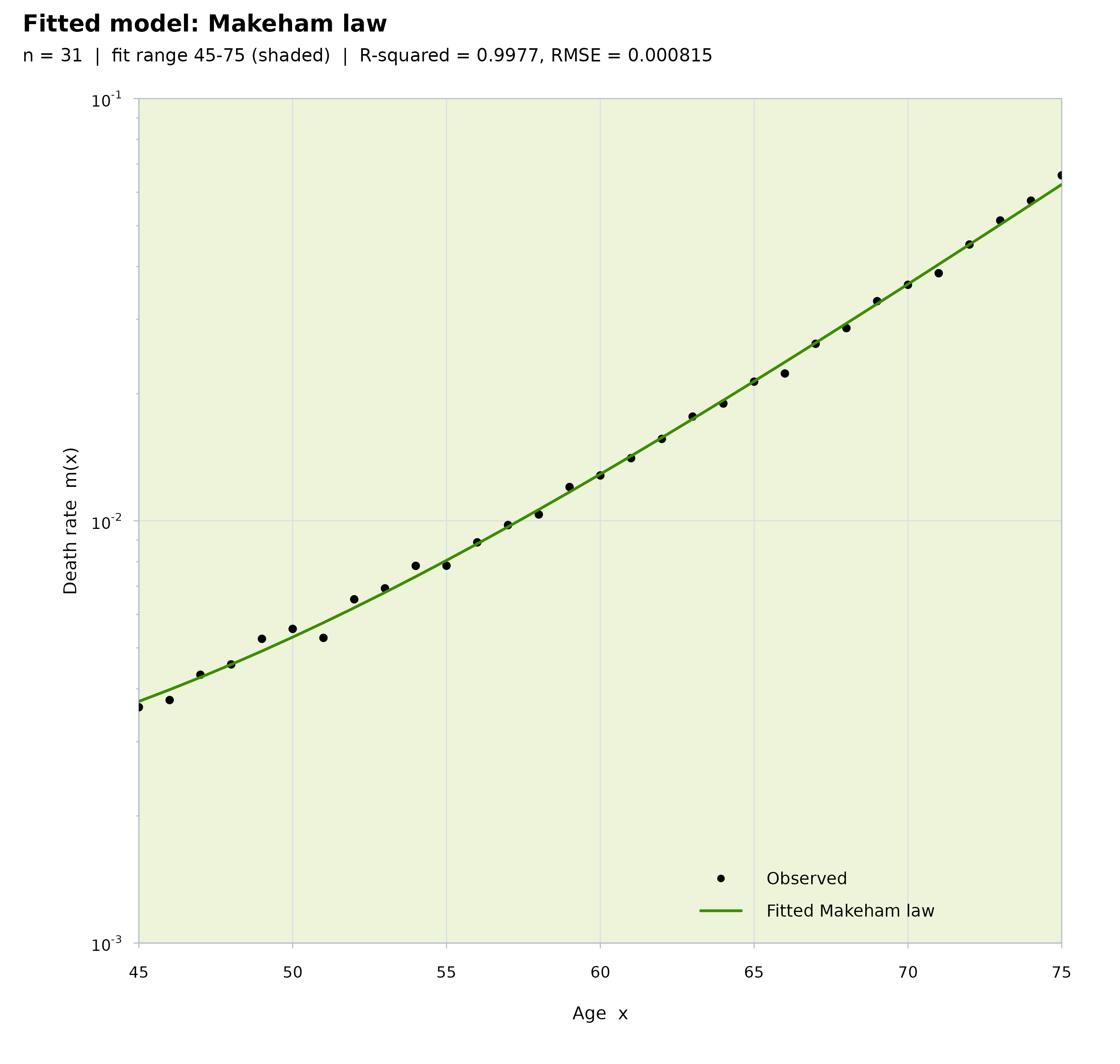
M1 <- MortalityLaw(x = x, Dx = Dx, Ex = Ex, law = 'makeham')
M1
#> Makeham model: mu[x] = A exp[Bx] + C
#> Fitted values: mx
ls(M1)
#> [1] "coefficients" "deviance" "deviance.residuals"
#> [4] "df" "dispersion" "fitted.values"
#> [7] "goodness.of.fit" "info" "input"
#> [10] "opt.diagnosis" "pearson.residuals" "residuals"
coef(M1)
#> A B C
#> 0.001850607 0.112722883 0.001663206
summary(M1)
#> Makeham model: mu[x] = A exp[Bx] + C
#> Fitted values: mx | ages 45-75 | fitted on 45-75 (31 of 31 ages)
#>
#> Call:
#> MortalityLaw(x = x, Dx = Dx, Ex = Ex, law = "makeham")
#>
#> Coefficients:
#> estimate
#> A 0.0019
#> B 0.1127
#> C 0.0017
#>
#> Fit:
#> method LF2 | optimiser converged in 21 iterations
#> deviance 117.3 on 28 degrees of freedom | dispersion 4.18
#> R-squared 0.9977 | RMSE 0.000815
#>
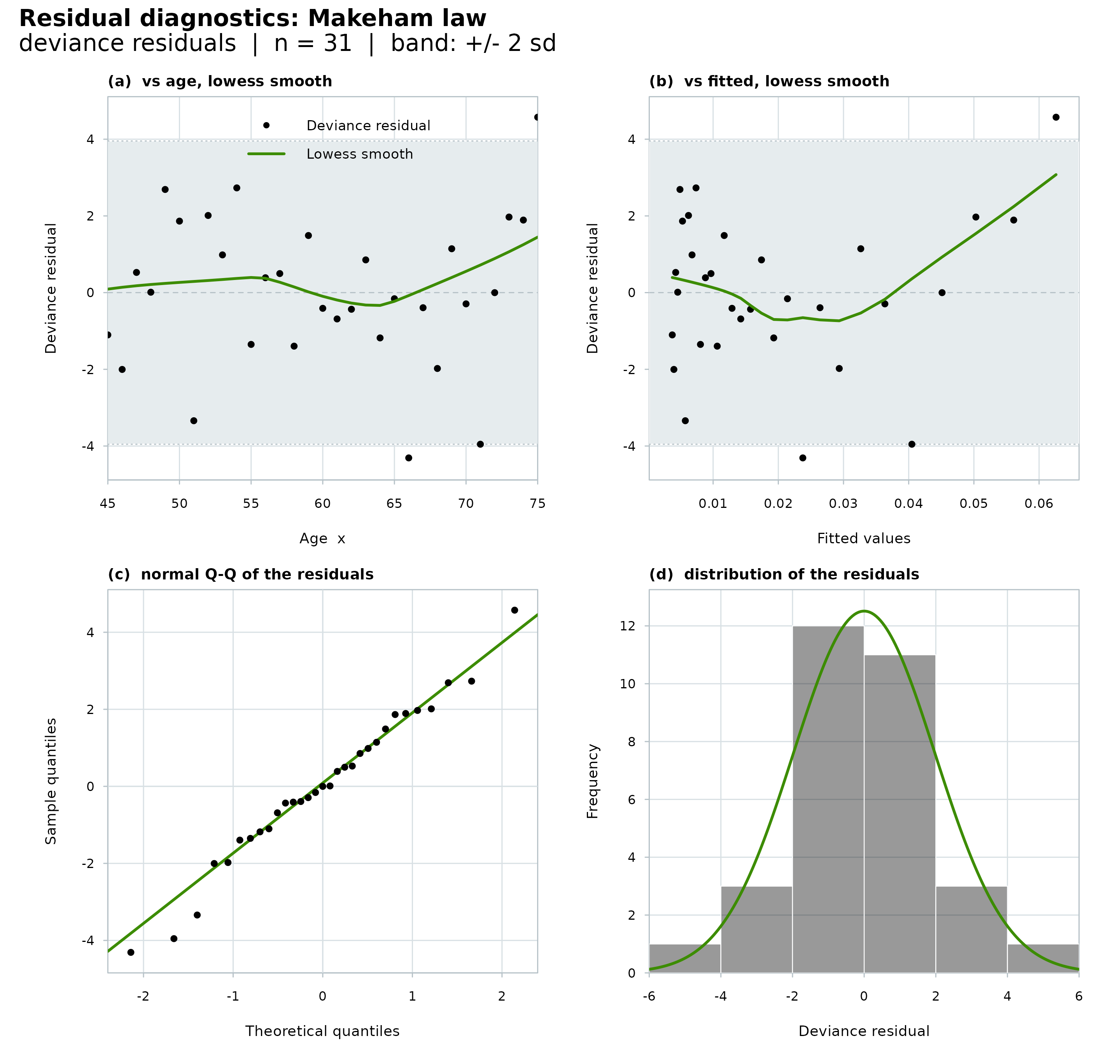
#> Residuals:
#> Min. 1st Qu. Median Mean 3rd Qu. Max.
#> raw -0.0019 -0.0002 0e+00 0.0001 0.0003 0.0032
#> deviance -4.3099 -1.1418 -9e-04 0.0204 1.3164 4.5737
fitted(M1)
#> 45 46 47 48 49 50
#> 0.003734630 0.003981796 0.004258454 0.004568123 0.004914743 0.005302722
#> 51 52 53 54 55 56
#> 0.005736995 0.006223087 0.006767180 0.007376195 0.008057878 0.008820901
#> 57 58 59 60 61 62
#> 0.009674970 0.010630947 0.011700994 0.012898720 0.014239360 0.015739968
#> 63 64 65 66 67 68
#> 0.017419632 0.019299715 0.021404134 0.023759655 0.026396241 0.029347429
#> 69 70 71 72 73 74
#> 0.032650758 0.036348246 0.040486924 0.045119436 0.050304708 0.056108695
#> 75
#> 0.062605224
predict(M1, x = 45:95)
#> 45 46 47 48 49 50
#> 0.003734630 0.003981796 0.004258454 0.004568123 0.004914743 0.005302722
#> 51 52 53 54 55 56
#> 0.005736995 0.006223087 0.006767180 0.007376195 0.008057878 0.008820901
#> 57 58 59 60 61 62
#> 0.009674970 0.010630947 0.011700994 0.012898720 0.014239360 0.015739968
#> 63 64 65 66 67 68
#> 0.017419632 0.019299715 0.021404134 0.023759655 0.026396241 0.029347429
#> 69 70 71 72 73 74
#> 0.032650758 0.036348246 0.040486924 0.045119436 0.050304708 0.056108695
#> 75 76 77 78 79 80
#> 0.062605224 0.069876929 0.078016307 0.087126890 0.097324562 0.108739039
#> 81 82 83 84 85 86
#> 0.121515510 0.135816492 0.151823891 0.169741320 0.189796687 0.212245096
#> 87 88 89 90 91 92
#> 0.237372086 0.265497272 0.296978404 0.332215917 0.371658031 0.415806445
#> 93 94 95
#> 0.465222724 0.520535437 0.582448157
plot(M1, which = 'fit')
 plot(M1, which = 'diagnostics')
 # Example 2: --------------------------
# We can fit the same model using a different data format
# and a different optimization method.
x <- 45:75
mx <- ahmd$mx[paste(x), ]
M2 <- MortalityLaw(x = x, mx = mx, law = 'makeham', opt.method = 'LF1')
M2
#> Makeham model: mu[x] = A exp[Bx] + C
#> Fitted values: mx
fitted(M2)
#> 1850 1900 1950 2010
#> 45 0.01268912 0.01195113 0.003719844 0.001385711
#> 46 0.01310240 0.01257962 0.003967062 0.001513453
#> 47 0.01356032 0.01326547 0.004243761 0.001653738
#> 48 0.01406772 0.01401393 0.004553458 0.001807797
#> 49 0.01462995 0.01483070 0.004900087 0.001976982
#> 50 0.01525292 0.01572202 0.005288052 0.002162780
#> 51 0.01594321 0.01669469 0.005722284 0.002366820
#> 52 0.01670807 0.01775614 0.006208300 0.002590895
#> 53 0.01755558 0.01891448 0.006752274 0.002836971
#> 54 0.01849466 0.02017853 0.007361119 0.003107209
#> 55 0.01953520 0.02155797 0.008042571 0.003403980
#> 56 0.02068817 0.02306330 0.008805288 0.003729891
#> 57 0.02196572 0.02470604 0.009658962 0.004087802
#> 58 0.02338130 0.02649871 0.010614440 0.004480856
#> 59 0.02494983 0.02845501 0.011683861 0.004912502
#> 60 0.02668783 0.03058986 0.012880815 0.005386531
#> 61 0.02861362 0.03291957 0.014220509 0.005907104
#> 62 0.03074749 0.03546192 0.015719966 0.006478790
#> 63 0.03311191 0.03823631 0.017398238 0.007106609
#> 64 0.03573181 0.04126393 0.019276650 0.007796072
#> 65 0.03863477 0.04456790 0.021379069 0.008553231
#> 66 0.04185139 0.04817343 0.023732209 0.009384734
#> 67 0.04541555 0.05210804 0.026365968 0.010297880
#> 68 0.04936482 0.05640178 0.029313812 0.011300686
#> 69 0.05374078 0.06108743 0.032613196 0.012401955
#> 70 0.05858956 0.06620074 0.036306042 0.013611355
#> 71 0.06396223 0.07178077 0.040439273 0.014939502
#> 72 0.06991541 0.07787010 0.045065406 0.016398057
#> 73 0.07651180 0.08451523 0.050243220 0.017999824
#> 74 0.08382092 0.09176687 0.056038506 0.019758865
#> 75 0.09191976 0.09968040 0.062524899 0.021690621
predict(M2, x = 55:90)
#> 1850 1900 1950 2010
#> 55 0.01953520 0.02155797 0.008042571 0.003403980
#> 56 0.02068817 0.02306330 0.008805288 0.003729891
#> 57 0.02196572 0.02470604 0.009658962 0.004087802
#> 58 0.02338130 0.02649871 0.010614440 0.004480856
#> 59 0.02494983 0.02845501 0.011683861 0.004912502
#> 60 0.02668783 0.03058986 0.012880815 0.005386531
#> 61 0.02861362 0.03291957 0.014220509 0.005907104
#> 62 0.03074749 0.03546192 0.015719966 0.006478790
#> 63 0.03311191 0.03823631 0.017398238 0.007106609
#> 64 0.03573181 0.04126393 0.019276650 0.007796072
#> 65 0.03863477 0.04456790 0.021379069 0.008553231
#> 66 0.04185139 0.04817343 0.023732209 0.009384734
#> 67 0.04541555 0.05210804 0.026365968 0.010297880
#> 68 0.04936482 0.05640178 0.029313812 0.011300686
#> 69 0.05374078 0.06108743 0.032613196 0.012401955
#> 70 0.05858956 0.06620074 0.036306042 0.013611355
#> 71 0.06396223 0.07178077 0.040439273 0.014939502
#> 72 0.06991541 0.07787010 0.045065406 0.016398057
#> 73 0.07651180 0.08451523 0.050243220 0.017999824
#> 74 0.08382092 0.09176687 0.056038506 0.019758865
#> 75 0.09191976 0.09968040 0.062524899 0.021690621
#> 76 0.10089366 0.10831622 0.069784817 0.023812052
#> 77 0.11083716 0.11774026 0.077910504 0.026141780
#> 78 0.12185502 0.12802446 0.087005206 0.028700259
#> 79 0.13406333 0.13924733 0.097184482 0.031509949
#> 80 0.14759071 0.15149455 0.108577670 0.034595515
#> 81 0.16257968 0.16485961 0.121329535 0.037984045
#> 82 0.17918816 0.17944455 0.135602102 0.041705287
#> 83 0.19759114 0.19536070 0.151576720 0.045791908
#> 84 0.21798250 0.21272956 0.169456365 0.050279784
#> 85 0.24057709 0.23168373 0.189468218 0.055208314
#> 86 0.26561295 0.25236792 0.211866551 0.060620763
#> 87 0.29335385 0.27494001 0.236935961 0.066564648
#> 88 0.32409208 0.29957233 0.264994981 0.073092148
#> 89 0.35815147 0.32645292 0.296400134 0.080260567
#> 90 0.39589088 0.35578699 0.331550456 0.088132835
# Example 3: --------------------------
# Now let's fit a mortality law that is not defined
# in the package, say a reparameterized Gompertz in
# terms of modal age at death
# hx = b*exp(b*(x-m)) (here b and m are the parameters to be estimated)
# A function with 'x' and 'par' as input has to be defined, which returns
# at least an object called 'hx' (hazard rate).
missov <- function(x, par = c(b = 0.13, M = 45)){
hx <- with(as.list(par), b*exp(b*(x - M)) )
return(as.list(environment()))
}
M3 <- MortalityLaw(x = x, Dx = Dx, Ex = Ex, custom.law = missov)
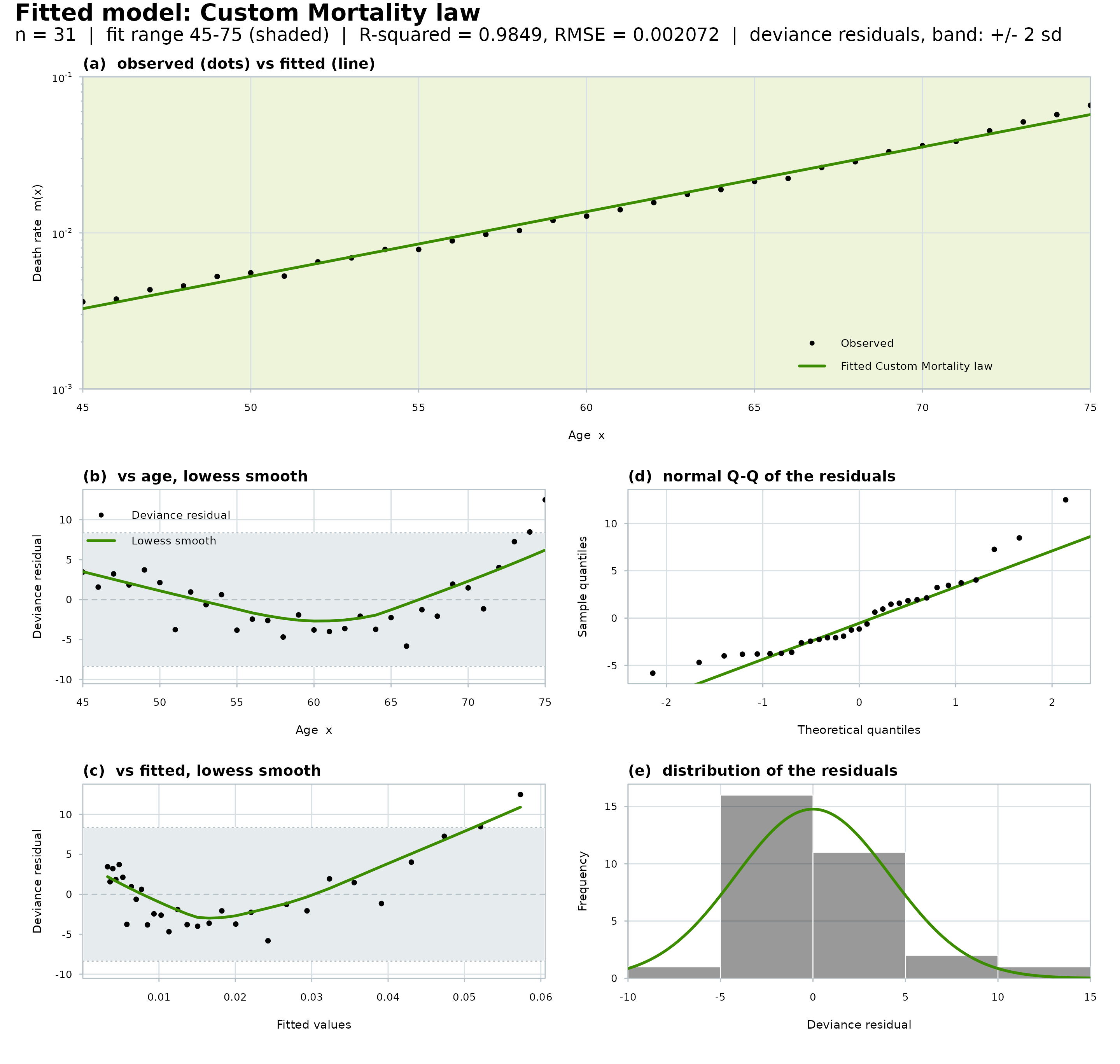
summary(M3)
#> Custom Mortality Law
#> Fitted values: mx | ages 45-75 | fitted on 45-75 (31 of 31 ages)
#>
#> Call:
#> MortalityLaw(x = x, Dx = Dx, Ex = Ex, custom.law = missov)
#>
#> Coefficients:
#> estimate
#> b 0.0955
#> M 36.3430
#>
#> Fit:
#> method LF2 | optimiser converged in 11 iterations
#> deviance 526 on 29 degrees of freedom | dispersion 18.45
#> R-squared 0.9849 | RMSE 0.002072
#>
#> Residuals:
#> Min. 1st Qu. Median Mean 3rd Qu. Max.
#> raw -0.0019 -0.0007 -0.0004 0.0003 0.0004 0.0085
#> deviance -5.8209 -3.1167 -1.1534 0.1143 2.0349 12.4956
plot(M3)
# Example 2: --------------------------
# We can fit the same model using a different data format
# and a different optimization method.
x <- 45:75
mx <- ahmd$mx[paste(x), ]
M2 <- MortalityLaw(x = x, mx = mx, law = 'makeham', opt.method = 'LF1')
M2
#> Makeham model: mu[x] = A exp[Bx] + C
#> Fitted values: mx
fitted(M2)
#> 1850 1900 1950 2010
#> 45 0.01268912 0.01195113 0.003719844 0.001385711
#> 46 0.01310240 0.01257962 0.003967062 0.001513453
#> 47 0.01356032 0.01326547 0.004243761 0.001653738
#> 48 0.01406772 0.01401393 0.004553458 0.001807797
#> 49 0.01462995 0.01483070 0.004900087 0.001976982
#> 50 0.01525292 0.01572202 0.005288052 0.002162780
#> 51 0.01594321 0.01669469 0.005722284 0.002366820
#> 52 0.01670807 0.01775614 0.006208300 0.002590895
#> 53 0.01755558 0.01891448 0.006752274 0.002836971
#> 54 0.01849466 0.02017853 0.007361119 0.003107209
#> 55 0.01953520 0.02155797 0.008042571 0.003403980
#> 56 0.02068817 0.02306330 0.008805288 0.003729891
#> 57 0.02196572 0.02470604 0.009658962 0.004087802
#> 58 0.02338130 0.02649871 0.010614440 0.004480856
#> 59 0.02494983 0.02845501 0.011683861 0.004912502
#> 60 0.02668783 0.03058986 0.012880815 0.005386531
#> 61 0.02861362 0.03291957 0.014220509 0.005907104
#> 62 0.03074749 0.03546192 0.015719966 0.006478790
#> 63 0.03311191 0.03823631 0.017398238 0.007106609
#> 64 0.03573181 0.04126393 0.019276650 0.007796072
#> 65 0.03863477 0.04456790 0.021379069 0.008553231
#> 66 0.04185139 0.04817343 0.023732209 0.009384734
#> 67 0.04541555 0.05210804 0.026365968 0.010297880
#> 68 0.04936482 0.05640178 0.029313812 0.011300686
#> 69 0.05374078 0.06108743 0.032613196 0.012401955
#> 70 0.05858956 0.06620074 0.036306042 0.013611355
#> 71 0.06396223 0.07178077 0.040439273 0.014939502
#> 72 0.06991541 0.07787010 0.045065406 0.016398057
#> 73 0.07651180 0.08451523 0.050243220 0.017999824
#> 74 0.08382092 0.09176687 0.056038506 0.019758865
#> 75 0.09191976 0.09968040 0.062524899 0.021690621
predict(M2, x = 55:90)
#> 1850 1900 1950 2010
#> 55 0.01953520 0.02155797 0.008042571 0.003403980
#> 56 0.02068817 0.02306330 0.008805288 0.003729891
#> 57 0.02196572 0.02470604 0.009658962 0.004087802
#> 58 0.02338130 0.02649871 0.010614440 0.004480856
#> 59 0.02494983 0.02845501 0.011683861 0.004912502
#> 60 0.02668783 0.03058986 0.012880815 0.005386531
#> 61 0.02861362 0.03291957 0.014220509 0.005907104
#> 62 0.03074749 0.03546192 0.015719966 0.006478790
#> 63 0.03311191 0.03823631 0.017398238 0.007106609
#> 64 0.03573181 0.04126393 0.019276650 0.007796072
#> 65 0.03863477 0.04456790 0.021379069 0.008553231
#> 66 0.04185139 0.04817343 0.023732209 0.009384734
#> 67 0.04541555 0.05210804 0.026365968 0.010297880
#> 68 0.04936482 0.05640178 0.029313812 0.011300686
#> 69 0.05374078 0.06108743 0.032613196 0.012401955
#> 70 0.05858956 0.06620074 0.036306042 0.013611355
#> 71 0.06396223 0.07178077 0.040439273 0.014939502
#> 72 0.06991541 0.07787010 0.045065406 0.016398057
#> 73 0.07651180 0.08451523 0.050243220 0.017999824
#> 74 0.08382092 0.09176687 0.056038506 0.019758865
#> 75 0.09191976 0.09968040 0.062524899 0.021690621
#> 76 0.10089366 0.10831622 0.069784817 0.023812052
#> 77 0.11083716 0.11774026 0.077910504 0.026141780
#> 78 0.12185502 0.12802446 0.087005206 0.028700259
#> 79 0.13406333 0.13924733 0.097184482 0.031509949
#> 80 0.14759071 0.15149455 0.108577670 0.034595515
#> 81 0.16257968 0.16485961 0.121329535 0.037984045
#> 82 0.17918816 0.17944455 0.135602102 0.041705287
#> 83 0.19759114 0.19536070 0.151576720 0.045791908
#> 84 0.21798250 0.21272956 0.169456365 0.050279784
#> 85 0.24057709 0.23168373 0.189468218 0.055208314
#> 86 0.26561295 0.25236792 0.211866551 0.060620763
#> 87 0.29335385 0.27494001 0.236935961 0.066564648
#> 88 0.32409208 0.29957233 0.264994981 0.073092148
#> 89 0.35815147 0.32645292 0.296400134 0.080260567
#> 90 0.39589088 0.35578699 0.331550456 0.088132835
# Example 3: --------------------------
# Now let's fit a mortality law that is not defined
# in the package, say a reparameterized Gompertz in
# terms of modal age at death
# hx = b*exp(b*(x-m)) (here b and m are the parameters to be estimated)
# A function with 'x' and 'par' as input has to be defined, which returns
# at least an object called 'hx' (hazard rate).
missov <- function(x, par = c(b = 0.13, M = 45)){
hx <- with(as.list(par), b*exp(b*(x - M)) )
return(as.list(environment()))
}
M3 <- MortalityLaw(x = x, Dx = Dx, Ex = Ex, custom.law = missov)
summary(M3)
#> Custom Mortality Law
#> Fitted values: mx | ages 45-75 | fitted on 45-75 (31 of 31 ages)
#>
#> Call:
#> MortalityLaw(x = x, Dx = Dx, Ex = Ex, custom.law = missov)
#>
#> Coefficients:
#> estimate
#> b 0.0955
#> M 36.3430
#>
#> Fit:
#> method LF2 | optimiser converged in 11 iterations
#> deviance 526 on 29 degrees of freedom | dispersion 18.45
#> R-squared 0.9849 | RMSE 0.002072
#>
#> Residuals:
#> Min. 1st Qu. Median Mean 3rd Qu. Max.
#> raw -0.0019 -0.0007 -0.0004 0.0003 0.0004 0.0085
#> deviance -5.8209 -3.1167 -1.1534 0.1143 2.0349 12.4956
plot(M3)
 # predict M3 for different ages
predict(M3, x = 85:130)
#> 85 86 87 88 89 90 91
#> 0.1489511 0.1638746 0.1802932 0.1983569 0.2182303 0.2400949 0.2641500
#> 92 93 94 95 96 97 98
#> 0.2906153 0.3197321 0.3517662 0.3870097 0.4257843 0.4684438 0.5153773
#> 99 100 101 102 103 104 105
#> 0.5670131 0.6238223 0.6863232 0.7550862 0.8307385 0.9139704 1.0055413
#> 106 107 108 109 110 111 112
#> 1.1062868 1.2171260 1.3390702 1.4732320 1.6208355 1.7832275 1.9618896
#> 113 114 115 116 117 118 119
#> 2.1584518 2.3747077 2.6126304 2.8743906 3.1623766 3.4792160 3.8277996
#> 120 121 122 123 124 125 126
#> 4.2113079 4.6332401 5.0974457 5.6081602 6.1700434 6.7882218 7.4683356
#> 127 128 129 130
#> 8.2165903 9.0398128 9.9455142 10.9419581
# Example 4: --------------------------
# Fit Heligman-Pollard model for a single
# year in the dataset between age 0 and 100 and build a life table.
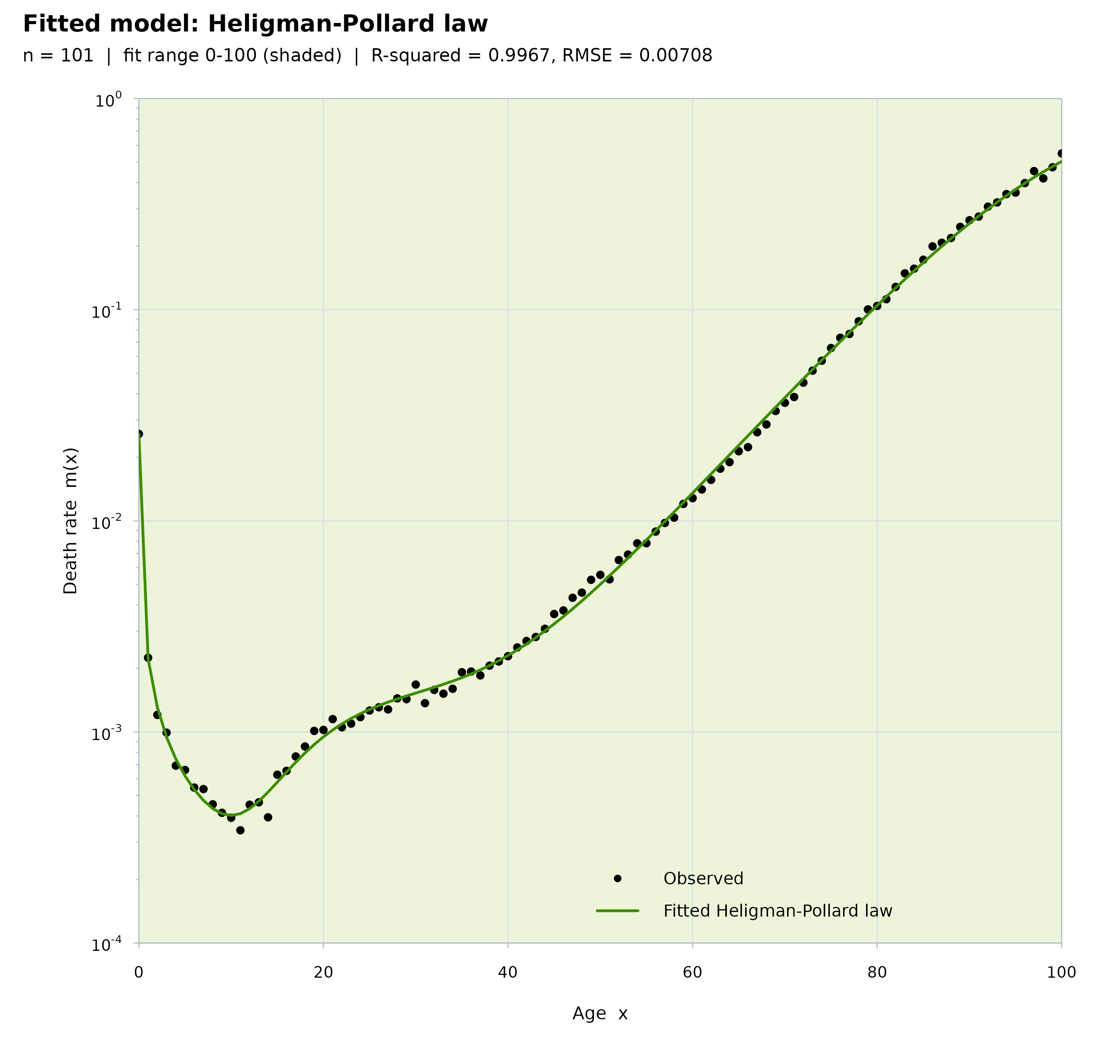
x <- 0:100
mx <- ahmd$mx[paste(x), "1950"] # select data
M4 <- MortalityLaw(x = x, mx = mx, law = 'HP', opt.method = 'LF2')
M4
#> Heligman-Pollard model: q[x]/p[x] = A^[(x + B)^C] + D exp[-E log(x/F)^2] + G H^x
#> Fitted values: mx
plot(M4, which = 'fit')
# predict M3 for different ages
predict(M3, x = 85:130)
#> 85 86 87 88 89 90 91
#> 0.1489511 0.1638746 0.1802932 0.1983569 0.2182303 0.2400949 0.2641500
#> 92 93 94 95 96 97 98
#> 0.2906153 0.3197321 0.3517662 0.3870097 0.4257843 0.4684438 0.5153773
#> 99 100 101 102 103 104 105
#> 0.5670131 0.6238223 0.6863232 0.7550862 0.8307385 0.9139704 1.0055413
#> 106 107 108 109 110 111 112
#> 1.1062868 1.2171260 1.3390702 1.4732320 1.6208355 1.7832275 1.9618896
#> 113 114 115 116 117 118 119
#> 2.1584518 2.3747077 2.6126304 2.8743906 3.1623766 3.4792160 3.8277996
#> 120 121 122 123 124 125 126
#> 4.2113079 4.6332401 5.0974457 5.6081602 6.1700434 6.7882218 7.4683356
#> 127 128 129 130
#> 8.2165903 9.0398128 9.9455142 10.9419581
# Example 4: --------------------------
# Fit Heligman-Pollard model for a single
# year in the dataset between age 0 and 100 and build a life table.
x <- 0:100
mx <- ahmd$mx[paste(x), "1950"] # select data
M4 <- MortalityLaw(x = x, mx = mx, law = 'HP', opt.method = 'LF2')
M4
#> Heligman-Pollard model: q[x]/p[x] = A^[(x + B)^C] + D exp[-E log(x/F)^2] + G H^x
#> Fitted values: mx
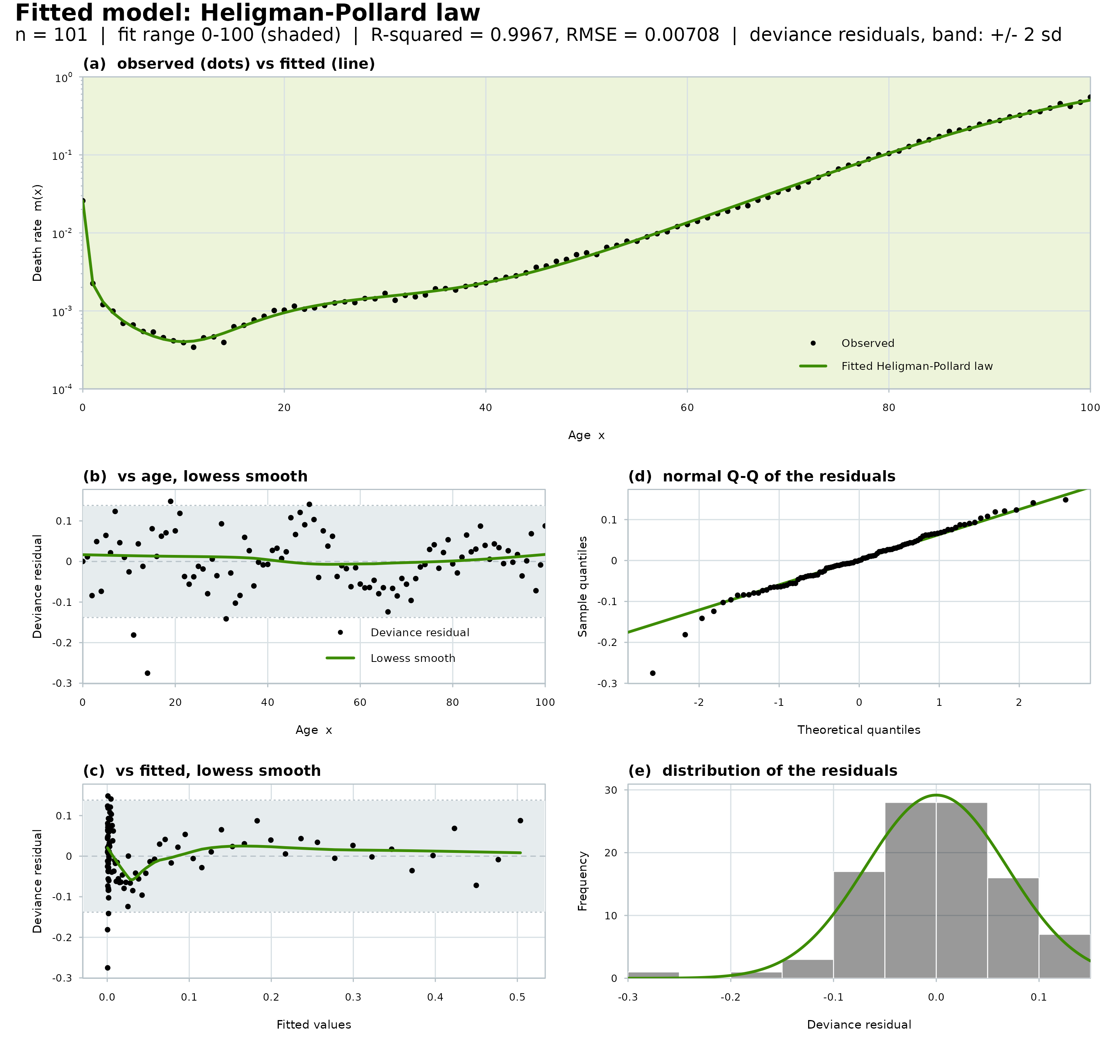
plot(M4, which = 'fit')
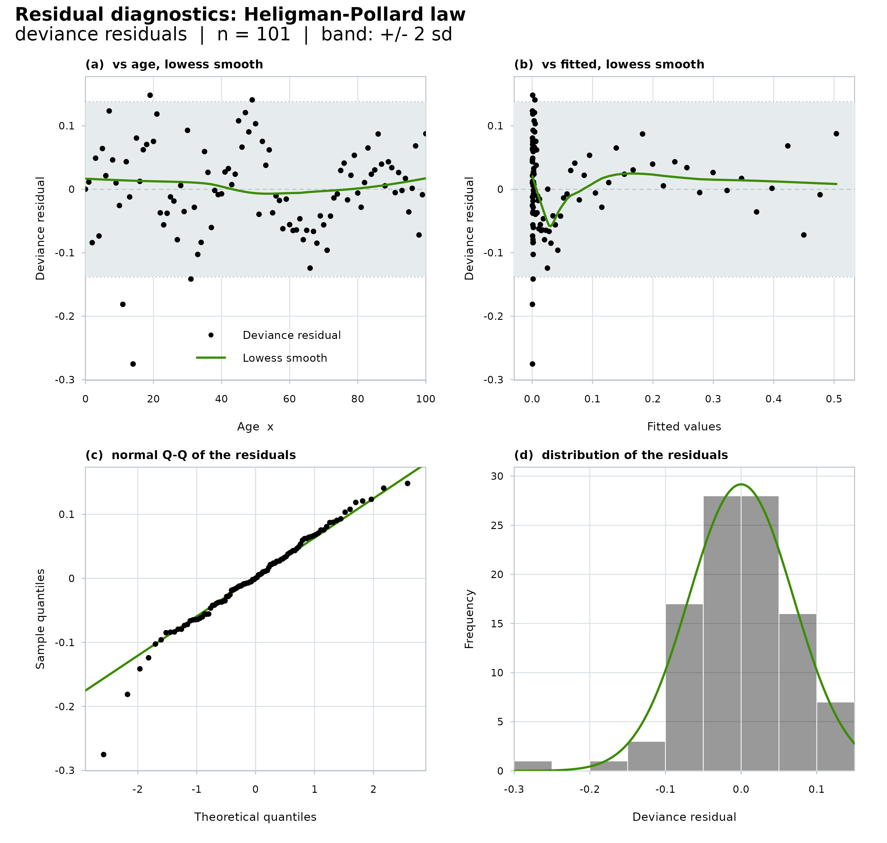
 plot(M4, which = 'diagnostics')
 plot(M4, which = 'both')
 LifeTable(x = x, qx = fitted(M4))
#> 'qx' is not closed at the last age; it has been set to 1. That is the usual way to close a life table and is applied here, so closing the input yourself is optional.
#>
#> Full Life Table
#>
#> Number of life tables: 1
#> Dimension: 101 x 10
#> Age intervals: [0,1) [1,2) [2,3) ... ... [98,99) [99,100) [100,+)
#>
#> x.int x mx qx ax lx dx Lx Tx ex
#> [0,1) 0 0.0264 0.0258 0.13 1e+05 2578 97761 7093734 70.94
#> [1,2) 1 0.0022 0.0022 0.5 97422 216 97314 6995972 71.81
#> [2,3) 2 0.0013 0.0013 0.5 97206 127 97142 6898659 70.97
#> [3,4) 3 9e-04 9e-04 0.5 97078 92 97033 6801516 70.06
#> [4,5) 4 7e-04 7e-04 0.5 96987 72 96951 6704484 69.13
#> [5,6) 5 6e-04 6e-04 0.5 96914 60 96884 6607533 68.18
#> <NA> ... ... ... ... ... ... ... ... ...
#> [98,99) 98 0.5805 0.4499 0.5 206 92 159 333 1.62
#> [99,100) 99 0.626 0.4768 0.5 113 54 86 174 1.54
#> [100,+) 100 0.6734 1 1.49 59 59 88 88 1.49
LifeTable(x = x, qx = fitted(M4))
#> 'qx' is not closed at the last age; it has been set to 1. That is the usual way to close a life table and is applied here, so closing the input yourself is optional.
#>
#> Full Life Table
#>
#> Number of life tables: 1
#> Dimension: 101 x 10
#> Age intervals: [0,1) [1,2) [2,3) ... ... [98,99) [99,100) [100,+)
#>
#> x.int x mx qx ax lx dx Lx Tx ex
#> [0,1) 0 0.0264 0.0258 0.13 1e+05 2578 97761 7093734 70.94
#> [1,2) 1 0.0022 0.0022 0.5 97422 216 97314 6995972 71.81
#> [2,3) 2 0.0013 0.0013 0.5 97206 127 97142 6898659 70.97
#> [3,4) 3 9e-04 9e-04 0.5 97078 92 97033 6801516 70.06
#> [4,5) 4 7e-04 7e-04 0.5 96987 72 96951 6704484 69.13
#> [5,6) 5 6e-04 6e-04 0.5 96914 60 96884 6607533 68.18
#> <NA> ... ... ... ... ... ... ... ... ...
#> [98,99) 98 0.5805 0.4499 0.5 206 92 159 333 1.62
#> [99,100) 99 0.626 0.4768 0.5 113 54 86 174 1.54
#> [100,+) 100 0.6734 1 1.49 59 59 88 88 1.49