Life tables and how `MortalityLaws` builds them
From deaths and rates to survivorship, person-years and life expectancy
Marius D. Pascariu
2026-10-05
Source:vignettes/Life-tables.Rmd
Life-tables.RmdA death rate is a fact about one year of one population. A life table turns a whole schedule of such facts into a statement about lives: how many of 100,000 newborns are still alive at each age, how many die at each age, and how many years remain on average at each age. That translation is mechanical once the conventions are fixed. This article is about the conventions, because that is where all the choices live.
MortalityLaws does the translation in one function,
LifeTable(). Hand it deaths and exposures, or rates, or
probabilities, or a survivorship curve, or a distribution of deaths, or
a curve of life expectancy, and it returns the full ten-column table.
Three points along the way ask for a decision: how rates become
probabilities (the \(a_x\) convention),
where the table closes (the open age group), and what to do when the
data stop before mortality does (closing and extending). We take those
in order, and finish with the two convenience wrappers,
convertFx() for one-off conversions and
LawTable() for tables that come from a parametric law
rather than from data.
The running example is ahmd, the bundled England and
Wales female data set: deaths, exposures and death rates at single ages
0 to 110 for the years 1850, 1900, 1950 and 2010. The rate series thins
out at the oldest ages (for 1900 the rows from age 107 on are missing),
so the examples below work on ages 0 to 105, where every year is
populated.
What a life table is
A life table follows one synthetic cohort of \(l_0\) newborns through life and records, for every age interval \([x, x+n)\), what happens to them. The cohort is synthetic in a precise sense: at every age it is exposed to the mortality that the real population showed at that age in one calendar year. The table is a summary of that year, not a forecast of anyone’s actual life.
LifeTable() returns an object of class
"LifeTable" with three parts: lt, the table
itself; call, the matched call; and
process_date, the timestamp. The lt data frame
has one row per age interval and ten columns:
| column | symbol | what it holds |
|---|---|---|
x.int |
the interval as a label, e.g. [0,1)
|
|
x |
\(x\) | the age at the start of the interval |
mx |
\(m_x\) | the death rate in \([x, x+n)\) |
qx |
\(q_x\) | the probability of dying within the interval |
ax |
\(a_x\) | the average years lived in the interval by those who die in it |
lx |
\(l_x\) | the survivors at exact age \(x\),
on the lx0 scale |
dx |
\(d_x\) | the deaths in the interval, on the same scale |
Lx |
\({}_nL_x\) | the person-years lived in the interval |
Tx |
\(T_x\) | the person-years remaining at age \(x\) |
ex |
\(e_x\) | the average years remaining, \(e_x = T_x / l_x\) |
The radix lx0 is 100,000 by default, so lx,
dx, Lx and Tx are counts in a
hypothetical population of 100,000 newborns. Set lx0 = 1
and the same columns read as survivorship probabilities instead. The
rates and probabilities do not depend on the choice.
The input can also be a matrix or a data frame with one column per
population or year. Each column then becomes its own table, stacked into
one lt with a leading LT column carrying the
column name, and plot() draws one curve per table.
The six ways in
Exactly one input case per call. Supplying two of them is an error, which is the kind of strictness that pays for itself the first time it fires.
| case | arguments | typical source |
|---|---|---|
| counts |
Dx and Ex
|
vital statistics over census exposures |
| rates | mx |
published rate series, e.g. the HMD |
| probabilities | qx |
published life tables |
| survivorship | lx |
published life tables |
| deaths | dx |
published life tables |
| expectancy | ex |
targets, forecasts, model outputs |
The count case
Given deaths and exposures, the rate \(m_x = D_x / E_x\) is computed for you and the rest of the table follows.
x  <- 0:105
Dx <- ahmd$Dx[as.character(x), "1900"]
Ex <- ahmd$Ex[as.character(x), "1900"]

lt_counts <- LifeTable(x = x, Dx = Dx, Ex = Ex)
head(lt_counts$lt, 4)
#>   x.int x         mx         qx      ax        lx        dx       Lx      Tx
#> 1 [0,1) 0 0.15130613 0.13693964 0.30663 100000.00 13693.964 90505.02 4825279
#> 2 [1,2) 1 0.04793397 0.04681202 0.50000  86306.04  4040.160 84285.96 4734774
#> 3 [2,3) 2 0.01912938 0.01894815 0.50000  82265.88  1558.786 81486.48 4650488
#> 4 [3,4) 3 0.01303322 0.01294883 0.50000  80707.09  1045.063 80184.56 4569001
#>         ex
#> 1 48.25279
#> 2 54.86028
#> 3 56.52997
#> 4 56.61214
Read the first row: 63,454 deaths in 419,375 person-years of exposure at age 0 give \(m_0 = 0.1513\). Of the 100,000 synthetic newborns, 13,694 die before their first birthday, and the 48.25 years of \(e_0\) are what the rest of the schedule adds up to.
The rate case
If the rates are already published, skip the division.
mx <- ahmd$mx[as.character(x), "1900"]

lt_rates <- LifeTable(x = x, mx = mx)
head(lt_rates$lt, 4)
#>   x.int x       mx         qx      ax        lx        dx       Lx      Tx
#> 1 [0,1) 0 0.151306 0.13693953 0.30663 100000.00 13693.953 90505.02 4825283
#> 2 [1,2) 1 0.047934 0.04681206 0.50000  86306.05  4040.163 84285.97 4734778
#> 3 [2,3) 2 0.019129 0.01894777 0.50000  82265.88  1558.755 81486.51 4650492
#> 4 [3,4) 3 0.013033 0.01294862 0.50000  80707.13  1045.046 80184.61 4569005
#>         ex
#> 1 48.25283
#> 2 54.86032
#> 3 56.53001
#> 4 56.61216
The two runs agree to the fourth decimal in \(e_0\) (48.25279 against 48.25283) but not
digit for digit, and the reason is worth knowing: the bundled
mx column is the published rate series, which is not
exactly Dx / Ex (the two differ by 0.016 at age 105, where
a handful of deaths sit on very small exposure). Which of the two you
treat as the source of truth is your decision, not the package’s.
Feeding columns back in
Each of the other four cases takes what a previous table produced. Feed any of the derived columns back and the same table comes out.
e0 <- c(
  DxEx = lt_counts$lt$ex[1],
  mx   = LifeTable(x = x, mx = lt_counts$lt$mx)$lt$ex[1],
  qx   = LifeTable(x = x, qx = lt_counts$lt$qx)$lt$ex[1],
  lx   = LifeTable(x = x, lx = lt_counts$lt$lx)$lt$ex[1],
  dx   = LifeTable(x = x, dx = lt_counts$lt$dx)$lt$ex[1],
  ex   = LifeTable(x = x, ex = lt_counts$lt$ex)$lt$ex[1]
)
e0
#>     DxEx       mx       qx       lx       dx       ex
#> 48.25279 48.25279 48.25279 48.25279 48.25279 48.25279
All six agree to within \(10^{-6}\)
of a year in \(e_0\), and the
ex round trip is exact to machine precision. The
ex case is the interesting one, because it runs the table
backwards; the section on the ex inverse
shows how.
From rates to probabilities
A rate is not a probability. The rate \(m_x = D_x / E_x\) can exceed 1 at old ages, while \(q_x\) is a probability and cannot. Turning one into the other needs an assumption about where inside the interval the deaths occur, and that assumption is \(a_x\): the average number of years lived in the interval by those who die in it.
With \(a_x\) in hand, the exact interval identity gives
\[ q_x = \frac{n \, m_x}{1 + (n - a_x) \, m_x} \]
which in code is qx = n*mx/(1+(n-ax)*mx), and its
inverse
\[ m_x = \frac{q_x}{a_x q_x + n (1 - q_x)}. \]
The textbook alternative assumes a constant force of mortality inside the interval, \(\mu = m_x\), which integrates to
\[ q_x = 1 - e^{-n m_x}, \]
in code 1-exp(-n*mx), with the inverse \(m_x = -\log(1 - q_x)/n\).
Which formula you get depends on the \(a_x\) method (see Choosing ax). Whenever an \(a_x\) is known before the conversion,
either because you supplied one or because the method builds the whole
\(a_x\) column first, the exact
identity is used, so that the mx, qx and
ax columns describe each other exactly. The exponential
form is what cfm, preston and
coale_demeny leave in place: those methods convert under a
constant force of mortality and adjust \(a_x\) afterwards.
The two agree closely at ordinary rates and part company at the edges:
lt <- lt_rates$lt
q_exact <- (1 * lt$mx) / (1 + (1 - lt$ax) * lt$mx)
q_cfm   <- 1 - exp(-1 * lt$mx)

round(data.frame(
  age     = lt$x[1:3],
  mx      = lt$mx[1:3],
  ax      = lt$ax[1:3],
  qx      = lt$qx[1:3],
  q_exact = q_exact[1:3],
  q_cfm   = q_cfm[1:3]
  ), 4)
#>   age     mx     ax     qx q_exact  q_cfm
#> 1   0 0.1513 0.3066 0.1369  0.1369 0.1404
#> 2   1 0.0479 0.5000 0.0468  0.0468 0.0468
#> 3   2 0.0191 0.5000 0.0189  0.0189 0.0189
At age 0 the constant force form gives 0.1404 against the exact 0.1369, and the gap only widens where the rate is large. This is why the exact identity is the default: it is the one relation that keeps all three columns consistent.
How the columns are built
Once \(q_x\) is settled the rest of the table is bookkeeping. Survivorship falls by the deaths, and everything else accumulates person-years:
\[ l_{x+n} = l_x \, (1 - q_x), \qquad l_0 = l_{x0} \]
\[ d_x = l_x - l_{x+n} \]
\[ {}_nL_x = n \, l_x - (n - a_x) \, d_x = a_x \, l_x + (n - a_x) \, l_{x+n} \]
\[ T_x = \sum_{t = x,\, x+n,\, \ldots}^{\omega} {}_nL_t \]
\[ e_x = \frac{T_x}{l_x} \]
\(T_x\) sums the person-years from age \(x\) to the open age \(\omega\), so it is a cumulative total and \(e_x\) is simply that total per survivor. In code the whole recursion fits in four lines:
lx = lx0 * c(1, cumprod(1 - qx))     dx = lx - lx_shifted
Lx = n*lx - (n - ax)*dx              Lx[N] = lx[N]/mx[N]  (open row)
Tx = rev(cumsum(rev(Lx)))            ex = Tx/lx,  ex[N] = ax[N]
We can check the person-years identity against the table we already built:
lt <- lt_rates$lt
Lx_hand <- 1 * lt$lx - (1 - lt$ax) * lt$dx

max(abs(Lx_hand - lt$Lx))
#> [1] 4.499734e-13
The two agree to the last digit. One thing this identity quietly says: \(L_x\) depends on \(a_x\) as much as \(q_x\) does, so a life table is only as good as its \(a_x\) convention.
The rates fed into these recursions are rarely raw. Published tables are graduated first, smoothed so that the columns move plausibly with age; the classic actuarial treatment is Forfar et al. (1988), and fitting a parametric law is one modern way to do the same job.
Choosing ax
\(a_x\) is the average number of
years lived inside the interval by a person who dies in it. It fixes how
the person-years column \({}_nL_x\) is
split between the survivors and the dying, and through that split it
shapes the whole table. LifeTable() offers four methods for
it, plus the option of supplying your own values. They differ only at
the edges of the age range: infant ages, wide intervals, and the open
interval. Everywhere else they converge on the midpoint of the
interval.
ax |
what it does | when to use it |
|---|---|---|
andreev_kingkade (default) |
\(a_0\) from the Andreev-Kingkade rule keyed on \(m_0\) and sex; \(n/2\) on the other one-year intervals; the constant-force value on wider ones; \(1/m_x\) on the open row; conversion via the exact identity | reproduces the HMD period life tables (Andreev and Kingkade (2015); Wilmoth et al. (2025)). Use it unless you have a reason not to. |
cfm |
constant force of mortality in every interval: \(a_x = n + 1/m_x - n/q_x\) | reproducing tables built on that assumption; quick comparisons |
preston |
cfm, with the Coale-Demeny West \(a_0\) and \(a_1\) for the first two intervals,
expressed in \(m_x\)
|
following the textbook treatment of infant separation (Preston et al. (2001)) |
coale_demeny |
cfm, with the original 1983 \(q_0\) rule for the first two intervals (the
PAS coefficients) |
matching Coale-Demeny regional model tables and PAS output (Coale et al. (1983)) |
cfm has history: the constant-force value \(a_x = n + 1/m_x - n/q_x\) was the package’s
default \(a_x\) method until v2.8.0,
when andreev_kingkade took over. It is still available by
name, and it is still the fallback inside the default rule for intervals
wider than a year.
The first two intervals of an abridged table show what separates them. The data below are a textbook abridged schedule: one-year intervals at 0 and 1, five-year intervals above.
x_ab  <- c(0, 1, seq(5, 110, by = 5))
mx_ab <- c(.053, .005, .001, .0012, .0018, .002, .003, .004,
           .004, .005, .006, .0093, .0129, .019, .031, .049,
           .084, .129, .180, .2354, .3085, .390, .478, .551)

LT_ax <- lapply(c("andreev_kingkade", "cfm", "preston", "coale_demeny"), function(a)
  LifeTable(x = x_ab, mx = mx_ab, sex = "female", ax = a))
names(LT_ax) <- c("andreev_kingkade", "cfm", "preston", "coale_demeny")

ax_cmp <- t(sapply(LT_ax, function(L) L$lt$ax[1:2]))
colnames(ax_cmp) <- c("a0", "a1")
round(ax_cmp, 3)
#>                     a0    a1
#> andreev_kingkade 0.252 1.993
#> cfm              0.496 1.993
#> preston          0.201 1.442
#> coale_demeny     0.203 1.441
preston and coale_demeny differ by a
thousandth of a year here and agree exactly once \(m_0\) reaches 0.107. Both collapse onto
cfm when sex is not given, because the
childhood rule is keyed on the sex of the population. The life
expectancies differ in the second decimal:
e0_ax <- sapply(LT_ax, function(L) L$lt$ex[1])
round(e0_ax, 2)
#> andreev_kingkade              cfm          preston     coale_demeny
#>            64.91            64.88            64.85            64.85
If you have your own \(a_x\) values, pass them instead: a scalar applies everywhere, a vector must have one value per age. A value an interval cannot support (\(a_x m_x > 1\), more person-years than the interval holds) is replaced with the implied average \(1/m_x\), and the affected ages are reported in a warning.
The open age group
Every life table must stop somewhere, and the last row is a
convention rather than a measurement. At the open age \(N\) (the + in
85+, or wherever you choose to close), the package applies
the standard reciprocal rule ax = ex = 1/mx:
\[ a_N = e_N = \frac{1}{m_N}, \qquad q_N = 1, \qquad {}_nL_N = \frac{l_N}{m_N}. \]
In words: everyone still in the table dies in the open interval, the interval lasts exactly \(1/m_N\) years on average, and life expectancy there equals that duration. (A life table always ends with an assumption; at least this one is printed in the last row.)
lt_ab <- LifeTable(x = x_ab, mx = mx_ab, sex = "female")
tail(lt_ab$lt, 2)
#>        x.int   x    mx        qx       ax       lx       dx         Lx
#> 23 [105,110) 105 0.478 0.9083703 1.587687 57.98012 52.66742 110.182882
#> 24   [110,+) 110 0.551 1.0000000 1.814882  5.31270  5.31270   9.641923
#>            Tx       ex
#> 23 119.824805 2.066653
#> 24   9.641923 1.814882
Read the last row of the abridged table: \(m_{110} = 0.551\), so \(a_{110} = e_{110} = 1/0.551 = 1.81\) years, and the 5,313 survivors at 110 contribute their \(9,642 = 5{,}313 / 0.551\) person-years to \(T_{110}\).
The rule assumes the force of mortality is roughly constant above the
open age. That holds when the open interval is old (85+ or 90+) and
fails when the data stop at 75+. The omega argument is the
clean fix when the data stop early: it extends the table to a later
closing age, filling the new rows by extrapolating a mortality law. How
that extrapolation works is the subject of the next section.
Closing and extending the table
Two arguments deal with a tail that the data do not reach, and they attack the problem from different sides.
close stays on the age grid you gave it and replaces the
open rate with the model-implied average force of mortality over the
open interval, \(1/e_N\) from the
fitted law. omega extends the age grid to a later closing
age and fills the added rows with the law’s rates. Both are named by a
mortality-law code from availableLaws(), both are fitted
from fit_from (age 60 when the input reaches 85, the last
20 years of the input otherwise), and when omega is set
without close the extrapolation defaults to
"kannisto", the standard old-age extension.
The example data stop at 75+:
x5  <- c(0, 1, seq(5, 75, by = 5))
mx5 <- c(.053, .005, .001, .0012, .0018, .002, .003, .004,
         .004, .005, .006, .0093, .0129, .019, .031, .049, .084)

lt_plain <- LifeTable(x = x5, mx = mx5)
lt_close <- LifeTable(x = x5, mx = mx5, close = "kannisto")
lt_ext   <- LifeTable(x = x5, mx = mx5, omega = 110)

c(plain = lt_plain$lt$ex[1], close = lt_close$lt$ex[1], omega = lt_ext$lt$ex[1])
#>    plain    close    omega
#> 66.55551 64.71610 65.16495
The default reciprocal close freezes the age-75 rate of 0.084 forever and hands back \(e_{75} = 1/0.084 = 11.9\) years. The fitted law knows better: it raises the open rate to 0.129 and drops \(e_{75}\) to 7.7 years, which moves \(e_0\) from 66.6 to 64.7. Extending the grid to 110 with the same law lands between the two at 65.2, because the closing assumption there applies five ages later. None of the three is wrong; they answer slightly different questions, and the arguments let you say which one you mean.
close also accepts any other law code, so the tail can
be closed with the same model you fitted to the whole age range. One
caveat lives in LawTable() as well: laws that scale the age
vector while fitting (the SCALE_X column of
availableLaws()$table says which) only produce valid tables
from the lower bound of their fitting range upwards.
convertFx: one indicator at a time
Often you want one column, not a table. convertFx()
converts a single indicator into another and returns a plain vector (or
the same matrix you supplied), tagged with the conversion so that
plot() can show it.
The grid of possibilities is five inputs by seven outputs:
| from to | mx |
qx |
dx |
lx |
Lx |
Tx |
ex |
|---|---|---|---|---|---|---|---|
mx |
table | table | table | table | table | table | |
qx |
table | table | table | table | table | table | |
dx |
table | table | direct | table | table | table | |
lx |
table | table | direct | table | table | table | |
ex |
table | table | table | table | table | table |
Thirty-five combinations. Only the dx to lx
pair and its reverse are direct arithmetic (a cumulative sum and a
difference); every other pair is answered by building the full life
table in between, so the conversion honours whatever ax,
lx0, close or omega you pass
through ....
ex_1900 <- convertFx(x = x, data = mx, from = "mx", to = "ex")
round(ex_1900[1:3], 2)     # subsetting returns plain numbers
#> [1] 48.25 54.86 56.53

dx_1900 <- convertFx(x = x, data = lt_rates$lt$lx, from = "lx", to = "dx")
max(abs(unclass(dx_1900) - lt_rates$lt$dx))
#> [1] 7.275958e-12
The first conversion is a whole life table under the hood, so its
values are identical to the ex column built earlier. The
second is arithmetic and matches the table’s own dx column
to machine precision. plot.convertFx() draws the conversion
as it happened, the input indicator in one panel and the output in the
other:
plot(ex_1900)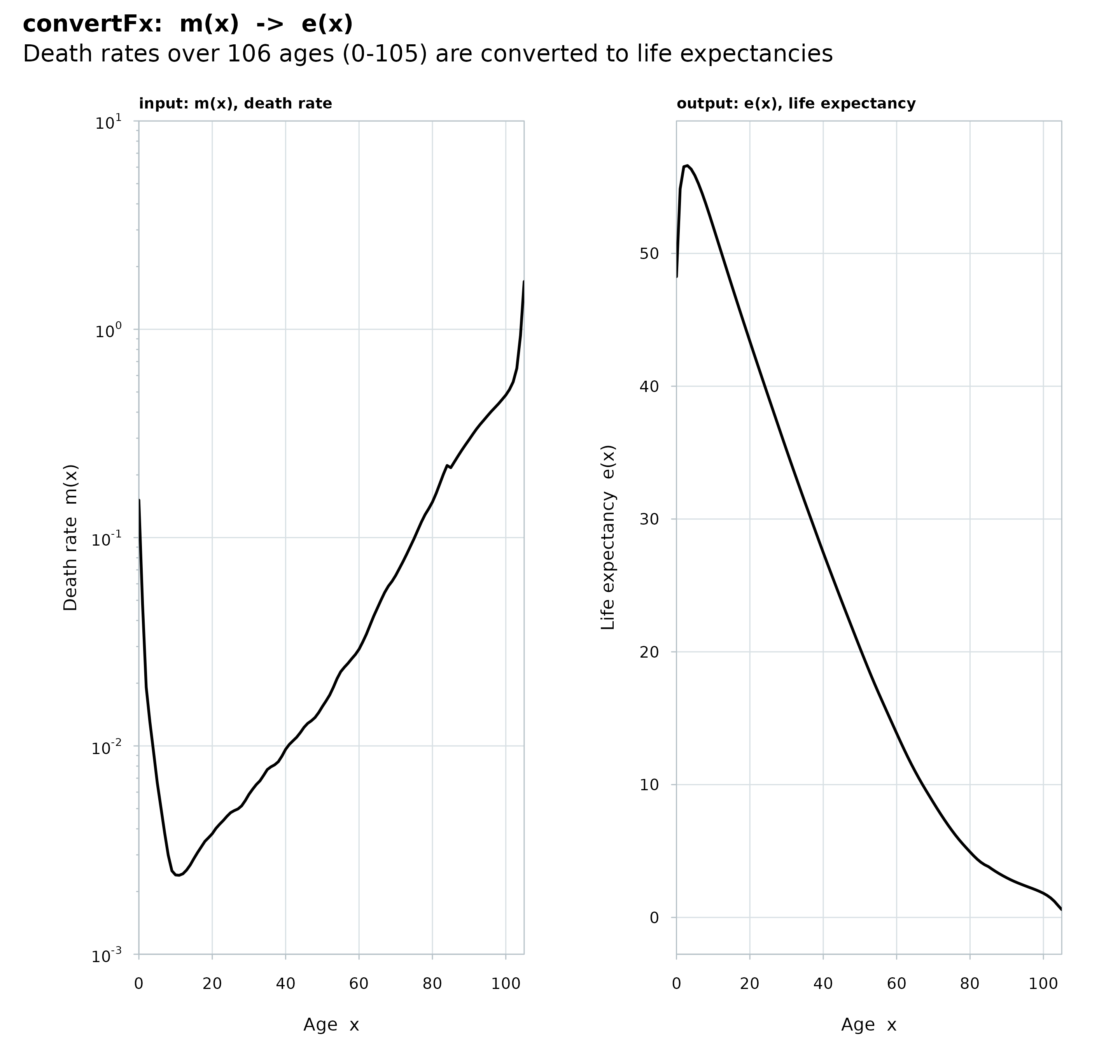
Rates and probabilities go on a log scale in whichever panel they appear, and a matrix input draws one curve per column.
LawTable: a table from a law
LawTable() takes the coefficients of a mortality law and
returns the life table the law implies. It is the natural next step
after a fit with MortalityLaw(), and the only thing to
watch is which scale the coefficients live on.
fit <- MortalityLaw(x = 60:100, mx = mx[x >= 60 & x <= 100], law = "gompertz")
coef(fit)
#>          A          B
#> 0.03065405 0.07179448

lt_law <- LawTable(x = 60:100, par = coef(fit), law = "gompertz")
round(head(lt_law$lt[, -1], 3), 4)
#>    x     mx     qx  ax        lx       dx       Lx      Tx      ex
#> 1 60 0.0329 0.0324 0.5 100000.00 3240.217 98379.89 1378829 13.7883
#> 2 61 0.0354 0.0348 0.5  96759.78 3364.539 95077.51 1280449 13.2333
#> 3 62 0.0380 0.0373 0.5  93395.24 3484.767 91652.86 1185372 12.6920
par may be a vector or a matrix with one row of
coefficients per table, and the law code must be one of the 38 in
availableLaws(). Laws that fit \(q_x\) (like the Heligman-Pollard family)
feed probabilities to LifeTable(), the rest feed rates. The
Gompertz above is one of the SCALE_X laws: it rescales the
age vector during fitting, so its coefficients refer to ages measured
from the start of the fitting range. Here the fit starts at 60 and the
table starts at 60, and the law puts \(e_{60}\) at 13.79 years against the 13.87
of the data table at the same age. Try the same coefficients at age 20
and the result would be quietly wrong; keep the lower bound of
x at the lower bound of the fit.
The ex inverse: a table from life expectancies
The ex input answers the question in reverse: given a
curve of remaining life expectancy, what life table produced it? The
method is the standard textbook inversion (Preston, Heuveline and
Guillot 2001, chapter 3, Preston et al. (2001)): it combines the interval
identity \({}_nL_x = a_x l_x + (n - a_x)
l_{x+n}\) with the \(T_x\)
recurrence, and both are relations the forward table is built on. The
\(a_x\) values it uses are the forward
table’s own rules: the Andreev-Kingkade \(a_0\) and the HMD protocol basis under the
default (Andreev and Kingkade (2015); Wilmoth et al. (2025)), the Coale-Demeny variant when
you ask for it (Coale et al. (1983)). The recovery rests on one
exact identity that holds for any \(a_x\):
\[ e_x \, l_x - e_{x+n} \, l_{x+n} = {}_nL_x = a_x \, l_x + (n - a_x) \, l_{x+n}. \]
Divide by \(l_x\) and the survivorship ratio of each closed interval falls out:
\[ r = \frac{l_{x+n}}{l_x} = \frac{e_x - a_x}{e_{x+n} + n - a_x} \]
which in code is:
r = (ex - ax)/(ex_n + n - ax)Then \(q_x = 1 - r\) and \(m_x = q_x / (a_x q_x + n (1 - q_x))\) follow, and the open interval closes by the usual rule, \(a_N = e_N\) and \(m_N = 1/e_N\).
There is one catch, and it is a real one: \(e_x\) alone does not pin down \(a_x\). Pass ax as a number and
the inversion is exact in one pass, because the ratios come straight
from the formula above. Leave it out and it turns into a fixed-point
problem: the default rule makes \(a_x\)
a function of the rate being recovered, so each interval must be solved
for the ratio \(r\) at which the \(a_x\) method in force reproduces it, that
is, the root of
\[ \frac{e_x - a(r)}{e_{x+n} + n - a(r)} - r = 0 \]
by bisection (120 iterations, on \(r \in (0, 1)\)). The root is unique: the left side is continuous and strictly decreasing in \(r\) for every method the package offers. The recovered table is then exactly the one the same \(e_x\) curve describes under that method.
lt_back <- LifeTable(x = x, ex = lt_rates$lt$ex)

round(data.frame(
  age    = x[1:3],
  ex_in  = lt_rates$lt$ex[1:3],
  ex_out = lt_back$lt$ex[1:3],
  mx_out = lt_back$lt$mx[1:3]
  ), 5)
#>   age    ex_in   ex_out  mx_out
#> 1   0 48.25283 48.25283 0.15131
#> 2   1 54.86032 54.86032 0.04793
#> 3   2 56.53001 56.53001 0.01913

max(abs(lt_back$lt$ex - lt_rates$lt$ex))
#> [1] 9.947598e-14
The round trip reproduces the input curve to \(10^{-13}\). The reverse is not guaranteed: not every curve of \(e_x\) is a feasible life table. A curve that rises at young ages is fine (when infant mortality is high, \(e_1 > e_0\)), but a value below its own \(a_x\), or falling faster than the interval width, gives death probabilities outside \([0, 1]\) and the function stops with the offending ages named. A missing value is an error too, never a repaired gap.
Reading the output
plot.LifeTable() draws the four classic panels:
survivorship \(l(x)\), the hazard \(m(x)\) on a log scale, the death
distribution \(d(x)\), and life
expectancy \(e(x)\).
lt_two <- LifeTable(
  x  = x,
  mx = ahmd$mx[as.character(x), c("1900", "2010")]
  )
plot(lt_two)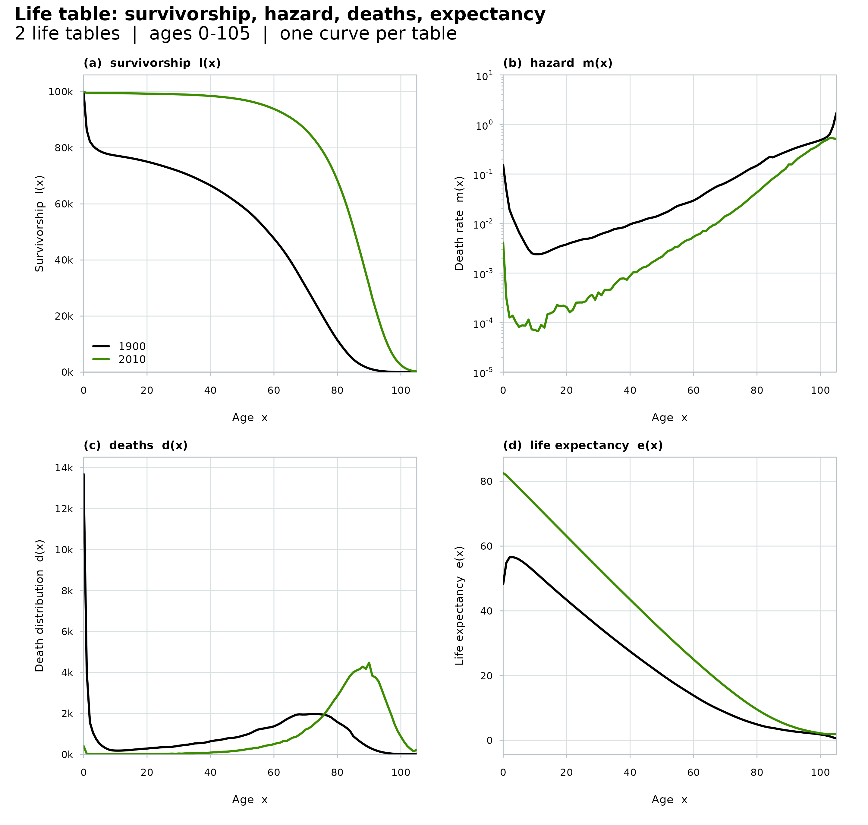
Two curves per panel, one per table. The 1900 curve shows the shape that used to be normal everywhere: heavy infant mortality, a young-adult hump, then the Gompertz rise. The 2010 curve has flattened at both ends. One number from each table captures most of it: \(e_0\) was 48.3 years in 1900 and 82.5 in 2010.
which selects a single panel and split
rearranges the layout:
plot(lt_two, which = "hazard")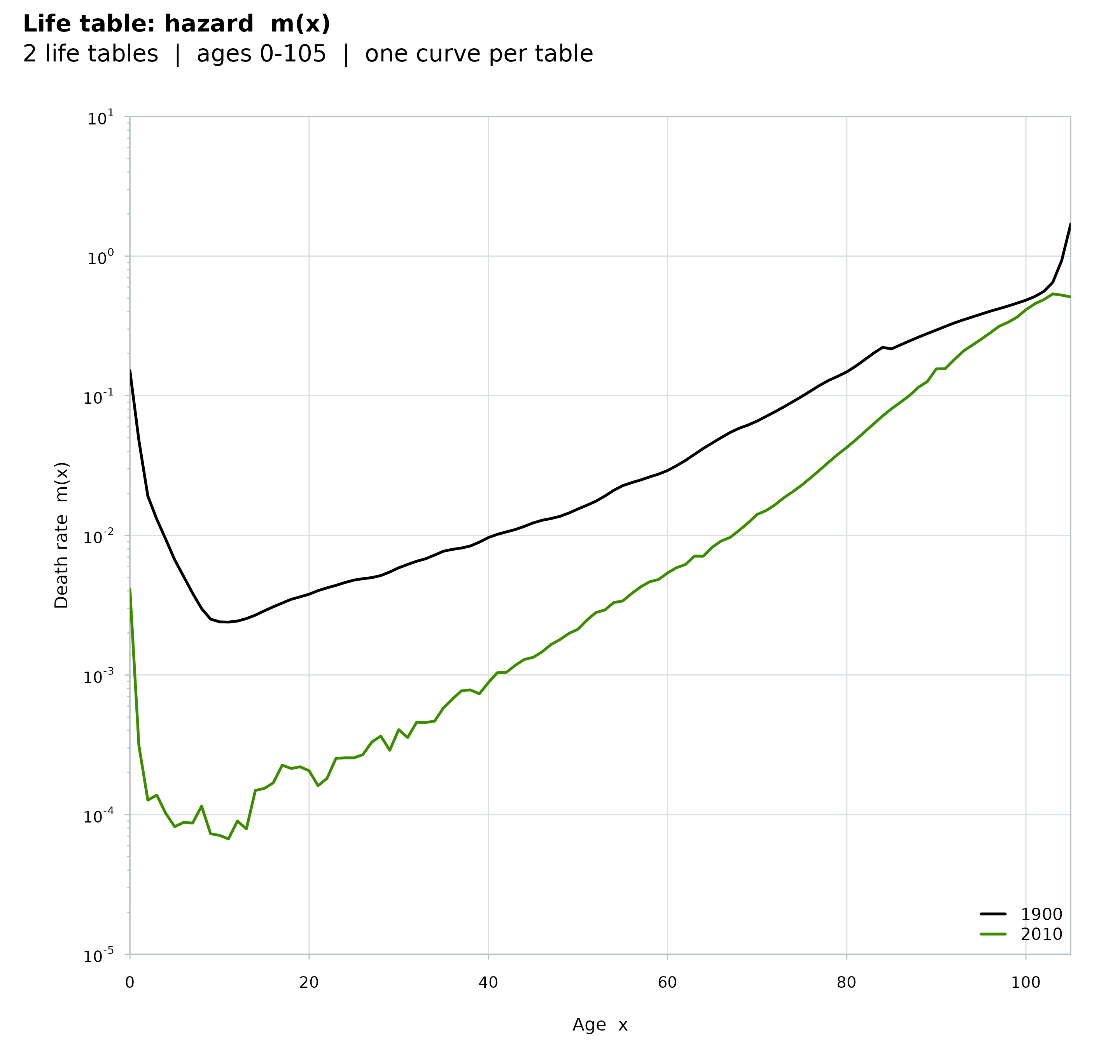
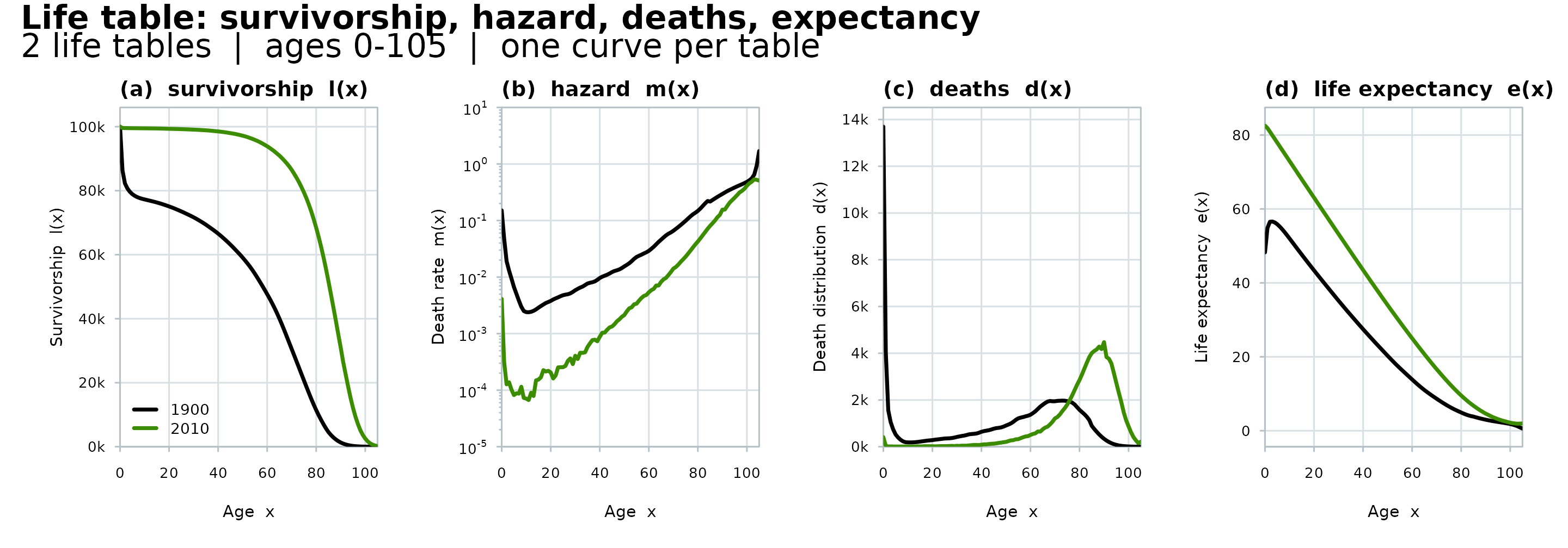
The which values are "all" (the default),
"lx", "hazard", "dx" and
"ex"; split takes a c(nrow, ncol)
pair that must hold exactly one slot per panel. The same four panels are
what a LawTable() object plots, since it returns a
"LifeTable" like any other.
Session info
sessionInfo()
#> R version 4.6.1 (2026-06-24)
#> Platform: x86_64-pc-linux-gnu
#> Running under: Ubuntu 24.04.5 LTS
#>
#> Matrix products: default
#> BLAS:   /usr/lib/x86_64-linux-gnu/openblas-pthread/libblas.so.3
#> LAPACK: /usr/lib/x86_64-linux-gnu/openblas-pthread/libopenblasp-r0.3.26.so;  LAPACK version 3.12.0
#>
#> locale:
#>  [1] LC_CTYPE=C.UTF-8       LC_NUMERIC=C           LC_TIME=C.UTF-8
#>  [4] LC_COLLATE=C.UTF-8     LC_MONETARY=C.UTF-8    LC_MESSAGES=C.UTF-8
#>  [7] LC_PAPER=C.UTF-8       LC_NAME=C              LC_ADDRESS=C
#> [10] LC_TELEPHONE=C         LC_MEASUREMENT=C.UTF-8 LC_IDENTIFICATION=C
#>
#> time zone: UTC
#> tzcode source: system (glibc)
#>
#> attached base packages:
#> [1] stats     graphics  grDevices utils     datasets  methods   base
#>
#> other attached packages:
#> [1] MortalityLaws_3.0.0
#>
#> loaded via a namespace (and not attached):
#>  [1] httr_1.4.9        cli_3.6.6         knitr_1.52        rlang_1.3.0
#>  [5] xfun_0.61         otel_0.2.0        textshaping_1.0.5 jsonlite_2.0.0
#>  [9] htmltools_0.5.9   ragg_1.5.2        sass_0.4.10       rmarkdown_2.32
#> [13] evaluate_1.0.5    jquerylib_0.1.4   fastmap_1.2.0     yaml_2.3.12
#> [17] lifecycle_1.0.5   compiler_4.6.1    fs_2.1.0          pbapply_1.7-5
#> [21] systemfonts_1.3.2 digest_0.6.39     R6_2.6.1          parallel_4.6.1
#> [25] bslib_0.12.0      tools_4.6.1       pkgdown_2.2.1     cachem_1.1.0
#> [29] desc_1.4.3