Fit univariate penalized composite link model (PCLM) to ungroup binned count data, e.g. age-at-death distributions grouped in age classes.
Arguments
- x
Vector containing the starting values of the input intervals/bins. For example: if we have 3 bins
[0,5), [5,10) and [10, 15),xwill be defined by the vector:c(0, 5, 10).- y
Vector with counts to be ungrouped. It must have the same dimension as
x.- nlast
Length of the last interval. In the example above
nlastwould be 5.- offset
Optional offset term to calculate smooth mortality rates. A vector of the same length as x and y, or one of the same length as the ungrouped output. See Rizzi et al. (2015) for further details.
- out.step
Length of estimated intervals in output. Values between 0.1 and 1 are accepted. Default: 1.
- ci.level
Confidence level, as a percentage rather than a proportion, so
95and not0.95. Values in[50.1, 99.9]are accepted. It sets the width of both interval pairs inci: the pointwiseconf_lowerandconf_upper, and the mass-preservinglowerandupperscenarios. Default:95.- verbose
Logical value. Indicates whether a progress bar should be shown or not. Default:
FALSE.- control
List of fitting controls, given by name. A misspelled entry is an error rather than being silently ignored. An unnamed entry is matched positionally, so
list(100)setslambdaand nothing else; naming every entry is strongly preferred. Any setting not supplied takes its default fromcontrol.pclmfor this function, orcontrol.pclm2Dforpclm2D. See those pages for the meaning and default of each oflambda,kr,deg,int.lambda,diff,opt.method,max.iterandtol.- omega
Closing age of the distribution. An alternative to
nlast: when it is given, the width of the last interval is taken asomega - max(x). Give one of the two, not both.- na.action
What to do with unobserved cells in
y."fail", the default, rejects them."omit"drops the matching rows and lets the smoothing penalty bridge the gap, which is how a surface with interior gaps or a missing year is handled. OnlyNAcounts as unobserved; infinite values are always an error.
Value
The output is a list with the following components:
- input
A list with arguments provided in input. Saved for convenience.
- fitted
The fitted values of the PCLM model.
- ci
A list with two kinds of interval and they are not interchangeable.
lowerandupperare the two mass-conserving scenarios: the distribution implied by a uniformly lower and a uniformly higher hazard, each rescaled so that it totalssum(fitted). Because the total is held fixed, the low scenario moves deaths towards older ages and the two curves crossfittedin the tail. They are therefore scenarios, not pointwise bounds, and they carry no coverage level.conf_lowerandconf_upperare the pointwise marginalci.levelinterval for the fitted values, computed asfitted * exp(-/+ qnorm * SE). These do satisfyconf_lower <= fitted <= conf_upperand they do not totalsum(fitted). Use the first pair as low and high inputs to a life table, the second as a pointwise error bar on the estimate.- goodness.of.fit
A list containing goodness of fit measures: standard errors, AIC and BIC.
- smoothPar
Estimated smoothing parameters. In the univariate model a named vector of
lambda,kranddeg. In the two-dimensional modellambdasplits intolambda.xfor the age axis andlambda.yfor the year axis, so the vector islambda.x, lambda.y, kr, deg.- bin.definition
Additional values to identify the bins limits and location in input and output objects.
- deep
A list of objects created in the fitting process. Useful in diagnosis of possible issues.
- call
An unevaluated function call, that is, an unevaluated expression which consists of the named function applied to the given arguments.
Details
The PCLM method is based on the composite link model, which extends standard generalized linear models. It implements the idea that the observed counts, interpreted as realizations from Poisson distributions, are indirect observations of a finer (ungrouped) but latent sequence. This latent sequence represents the distribution of expected means on a fine resolution and has to be estimated from the aggregated data. Estimates are obtained by maximizing a penalized likelihood. This maximization is performed efficiently by a version of the iteratively reweighted least-squares algorithm. Optimal values of the smoothing parameter are chosen by minimizing Bayesian or Akaike's Information Criterion.
References
Rizzi S, Gampe J, Eilers PHC (2015). “Efficient Estimation of Smooth Distributions From Coarsely Grouped Data.” American Journal of Epidemiology, 182(2), 138-147. doi:10.1093/aje/kwv020 .
Examples
# Data
x <- c(0, 1, seq(5, 85, by = 5))
y <- c(294, 66, 32, 44, 170, 284, 287, 293, 361, 600, 998,
1572, 2529, 4637, 6161, 7369, 10481, 15293, 39016)
offset <- c(114, 440, 509, 492, 628, 618, 576, 580, 634, 657,
631, 584, 573, 619, 530, 384, 303, 245, 249) * 1000
nlast <- 26 # the size of the last interval
# Example 1 ----------------------
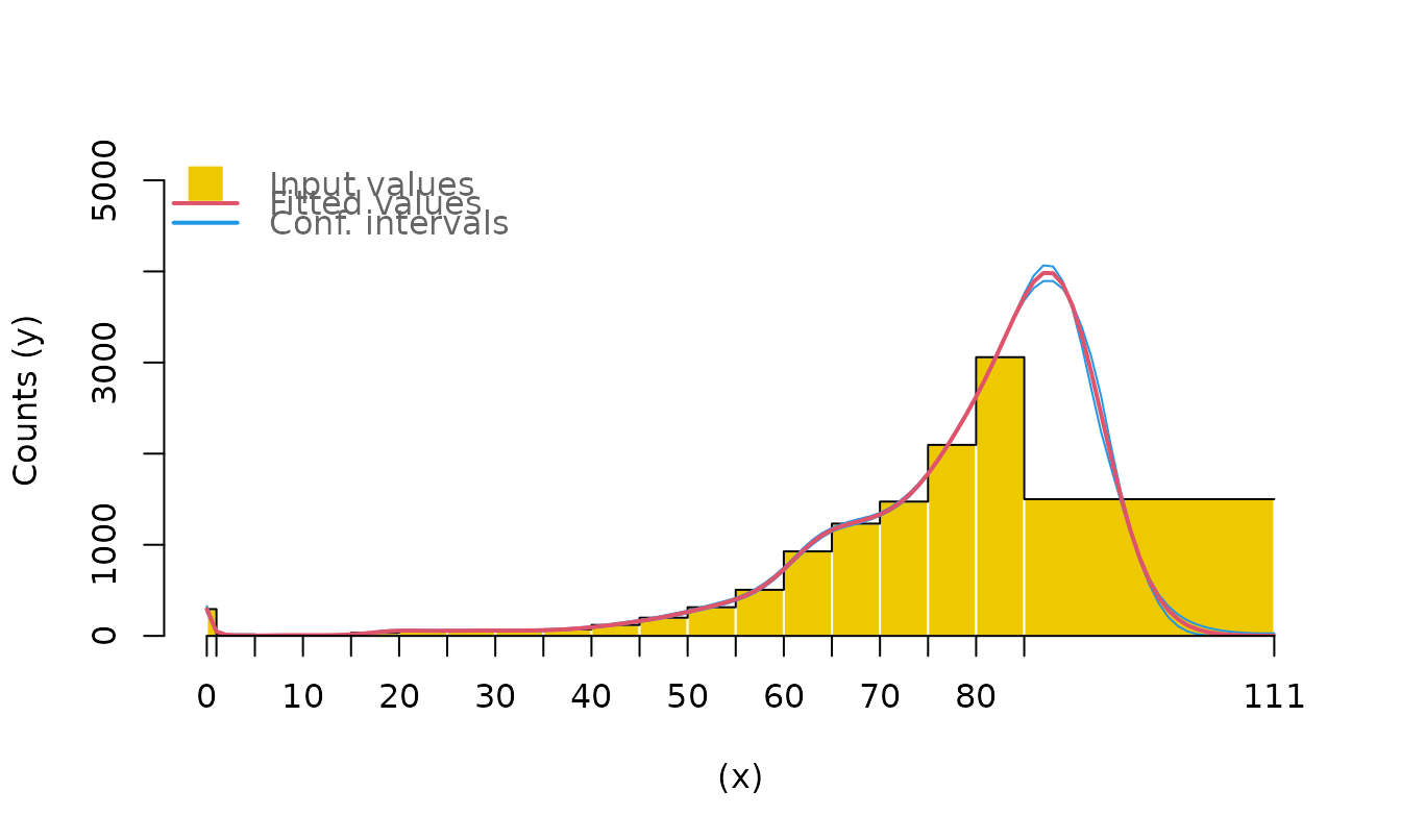
M1 <- pclm(x, y, nlast)
ls(M1)
#> [1] "bin.definition" "call" "ci" "deep"
#> [5] "fitted" "goodness.of.fit" "input" "smoothPar"
summary(M1)
#>
#> Penalized Composite Link Model (PCLM)
#>
#> Call:
#> pclm(x = x, y = y, nlast = nlast)
#>
#> PCLM Type : Univariate
#> Number of input groups : 19
#> Number of fitted values : 111
#> Length of estimate bins : 1
#> Smoothing parameter lambda : 0.1
#> B-splines intervals/knot (kr): 2
#> B-splines degree (deg) : 3
#> AIC : 39.97
#> BIC : 59.81
fitted(M1)
#> [0,1) [1,2) [2,3) [3,4) [4,5) [5,6)
#> 292.254945 47.567040 12.031104 5.101512 3.653694 3.801854
#> [6,7) [7,8) [8,9) [9,10) [10,11) [11,12)
#> 4.815457 6.352663 7.702012 8.349355 8.188017 7.844892
#> [12,13) [13,14) [14,15) [15,16) [16,17) [17,18)
#> 7.985346 9.025702 11.568904 16.221280 23.582754 33.474380
#> [18,19) [19,20) [20,21) [21,22) [22,23) [23,24)
#> 43.922241 52.410476 56.932803 57.933128 57.243741 56.233473
#> [24,25) [25,26) [26,27) [27,28) [28,29) [29,30)
#> 55.838792 56.123535 56.825906 57.606178 58.115022 58.277037
#> [30,31) [31,32) [32,33) [33,34) [34,35) [35,36)
#> 58.166052 58.010385 58.102700 58.696747 60.036110 62.332101
#> [36,37) [37,38) [38,39) [39,40) [40,41) [41,42)
#> 65.807514 70.655621 77.070029 85.156572 94.920752 106.255362
#> [42,43) [43,44) [44,45) [45,46) [46,47) [47,48)
#> 118.899308 132.628986 147.270502 162.850021 179.626932 197.884008
#> [48,49) [49,50) [50,51) [51,52) [52,53) [53,54)
#> 217.908603 239.747591 263.142589 287.749013 313.174561 339.648841
#> [54,55) [55,56) [56,57) [57,58) [58,59) [59,60)
#> 368.253616 401.033766 441.270637 492.262928 557.117381 637.375129
#> [60,61) [61,62) [62,63) [63,64) [64,65) [65,66)
#> 731.255969 833.938220 936.476422 1029.409950 1105.860969 1163.069720
#> [66,67) [67,68) [68,69) [69,70) [70,71) [71,72)
#> 1204.488941 1235.701765 1263.485202 1294.268889 1333.474545 1385.809083
#> [72,73) [73,74) [74,75) [75,76) [76,77) [77,78)
#> 1454.810931 1543.184019 1651.740928 1780.116411 1925.536315 2084.766185
#> [78,79) [79,80) [80,81) [81,82) [82,83) [83,84)
#> 2255.232116 2435.332561 2626.617486 2830.882343 3049.000300 3278.429175
#> [84,85) [85,86) [86,87) [87,88) [88,89) [89,90)
#> 3508.095452 3720.392828 3888.451678 3983.178893 3979.668950 3861.687654
#> [90,91) [91,92) [92,93) [93,94) [94,95) [95,96)
#> 3628.237712 3292.607166 2882.269883 2431.775913 1977.636196 1550.974452
#> [96,97) [97,98) [98,99) [99,100) [100,101) [101,102)
#> 1174.299714 859.519260 609.244616 418.991695 280.160080 182.530429
#> [102,103) [103,104) [104,105) [105,106) [106,107) [107,108)
#> 116.138627 72.331820 44.198811 26.560956 15.734729 9.210650
#> [108,109) [109,110) [110,111)
#> 5.340380 3.074238 1.761168
plot(M1)
 # Example 2 ----------------------
# ungroup even in smaller intervals
M2 <- pclm(x, y, nlast, out.step = 0.5)
head(fitted(M2))
#> [0,0.5) [0.5,1) [1,1.5) [1.5,2) [2,2.5) [2.5,3)
#> 211.751309 80.583507 32.679933 14.663354 7.463174 4.379770
plot(M2, type = "s")
# Example 2 ----------------------
# ungroup even in smaller intervals
M2 <- pclm(x, y, nlast, out.step = 0.5)
head(fitted(M2))
#> [0,0.5) [0.5,1) [1,1.5) [1.5,2) [2,2.5) [2.5,3)
#> 211.751309 80.583507 32.679933 14.663354 7.463174 4.379770
plot(M2, type = "s")
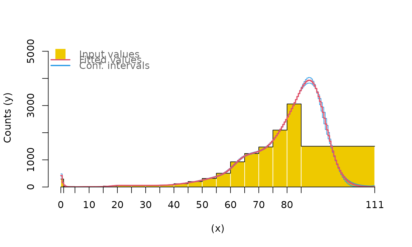 # Note, in example 1 we are estimating intervals of length 1. In example 2
# we are estimating intervals of length 0.5 using the same aggregate data.
# Example 3 ----------------------
# Do not optimise smoothing parameters; choose your own. Faster.
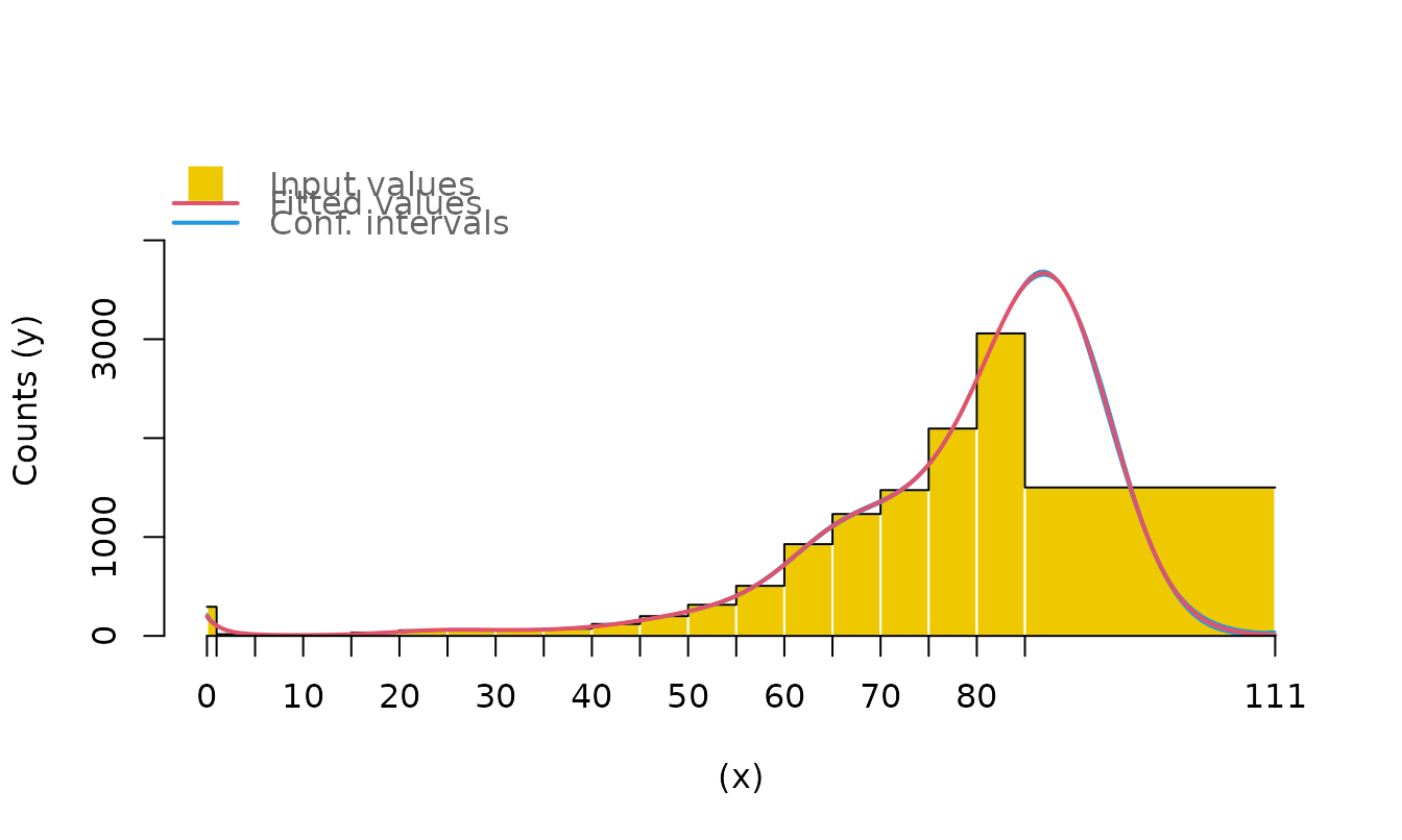
M3 <- pclm(x, y, nlast, out.step = 0.5,
control = list(lambda = 100, kr = 10, deg = 10))
plot(M3)
# Note, in example 1 we are estimating intervals of length 1. In example 2
# we are estimating intervals of length 0.5 using the same aggregate data.
# Example 3 ----------------------
# Do not optimise smoothing parameters; choose your own. Faster.
M3 <- pclm(x, y, nlast, out.step = 0.5,
control = list(lambda = 100, kr = 10, deg = 10))
plot(M3)
 summary(M2)
#>
#> Penalized Composite Link Model (PCLM)
#>
#> Call:
#> pclm(x = x, y = y, nlast = nlast, out.step = 0.5)
#>
#> PCLM Type : Univariate
#> Number of input groups : 19
#> Number of fitted values : 222
#> Length of estimate bins : 0.5
#> Smoothing parameter lambda : 7.732
#> B-splines intervals/knot (kr): 2
#> B-splines degree (deg) : 3
#> AIC : 39.96
#> BIC : 59.8
summary(M3) # not the smallest BIC here, but sometimes is not important.
#>
#> Penalized Composite Link Model (PCLM)
#>
#> Call:
#> pclm(x = x, y = y, nlast = nlast, out.step = 0.5, control = list(lambda = 100,
#> kr = 10, deg = 10))
#>
#> PCLM Type : Univariate
#> Number of input groups : 19
#> Number of fitted values : 222
#> Length of estimate bins : 0.5
#> Smoothing parameter lambda : 100
#> B-splines intervals/knot (kr): 10
#> B-splines degree (deg) : 10
#> AIC : 255.87
#> BIC : 267.49
# Example 4 -----------------------
# Grouped x & grouped offset (estimate death rates)
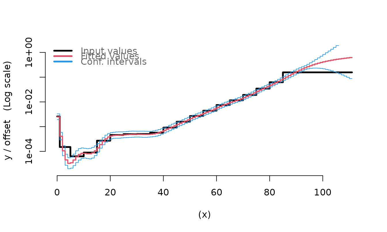
M4 <- pclm(x, y, nlast, offset)
plot(M4, type = "s")
summary(M2)
#>
#> Penalized Composite Link Model (PCLM)
#>
#> Call:
#> pclm(x = x, y = y, nlast = nlast, out.step = 0.5)
#>
#> PCLM Type : Univariate
#> Number of input groups : 19
#> Number of fitted values : 222
#> Length of estimate bins : 0.5
#> Smoothing parameter lambda : 7.732
#> B-splines intervals/knot (kr): 2
#> B-splines degree (deg) : 3
#> AIC : 39.96
#> BIC : 59.8
summary(M3) # not the smallest BIC here, but sometimes is not important.
#>
#> Penalized Composite Link Model (PCLM)
#>
#> Call:
#> pclm(x = x, y = y, nlast = nlast, out.step = 0.5, control = list(lambda = 100,
#> kr = 10, deg = 10))
#>
#> PCLM Type : Univariate
#> Number of input groups : 19
#> Number of fitted values : 222
#> Length of estimate bins : 0.5
#> Smoothing parameter lambda : 100
#> B-splines intervals/knot (kr): 10
#> B-splines degree (deg) : 10
#> AIC : 255.87
#> BIC : 267.49
# Example 4 -----------------------
# Grouped x & grouped offset (estimate death rates)
M4 <- pclm(x, y, nlast, offset)
plot(M4, type = "s")
 # Example 5 -----------------------
# Grouped x & ungrouped offset (estimate death rates)
ungroupped_Ex <- pclm(x, y = offset, nlast, offset = NULL)$fitted # ungroupped offset data
M5 <- pclm(x, y, nlast, offset = ungroupped_Ex)
# Example 5 -----------------------
# Grouped x & ungrouped offset (estimate death rates)
ungroupped_Ex <- pclm(x, y = offset, nlast, offset = NULL)$fitted # ungroupped offset data
M5 <- pclm(x, y, nlast, offset = ungroupped_Ex)