Introduction to ungroup

library(ungroup)

The problem

Demographers, actuaries, epidemiologists and criminologists all keep running into the same obstacle. The data are counts over intervals, and the intervals are too wide for the question being asked.

The bins are too coarse. Deaths are published in five-year age groups, and you need single years of age to compute an average age at death or to feed a model that expects an annual grid.
Different sources bin differently. One country publishes 5-year groups, another 10-year groups, a third has a wide open interval at the top. Any comparison between them is a comparison of the binning as much as of the underlying mortality.
The last interval is wide and open-ended. Ages “85 and over” can hold a third of the deaths in a low-mortality population. Treated as a single point it drags the tail, and every summary measure built on it inherits the distortion.

Spreading each bin’s count evenly over its width is the obvious move, and it is the one that goes wrong. It imposes a flat step on every interval, so the ungrouped sequence is a histogram of a histogram: no smoother than the input and wrong exactly where the data are most informative. The figure later in this vignette puts a number on that.

ungroup instead treats the coarse counts as indirect observations of a smooth underlying sequence and recovers it.

The model in one page

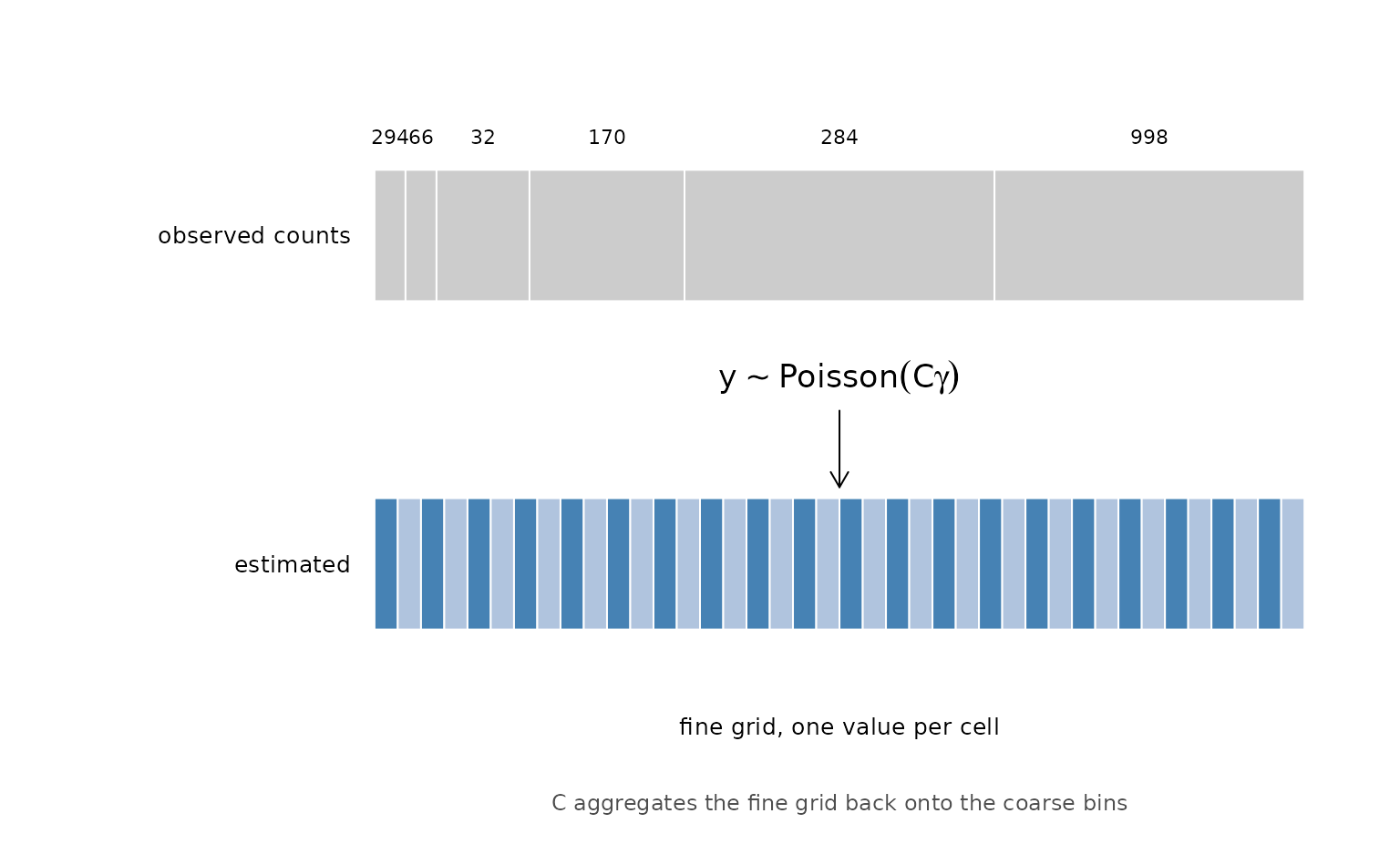
Write $y_i$ for the count in coarse interval $i$, $i = 1, \ldots, n$, and $\gamma_j$ for the expected mean on the fine grid $j = 1, \ldots, m$ that we want, with $m \gg n$. The observation is a sum, not a sample:

\[ y_i \sim \text{Poisson}\!\left(\sum_{j \in \mathcal{B}_i} \gamma_j\right) \]

where $\mathcal{B}_i$ is the set of fine cells falling inside coarse interval $i$. In matrix form $y \sim \text{Poisson}(C\gamma)$, where $C$ is a composition matrix of ones and zeros that maps the fine grid onto the coarse one. This is the composite link model of Thompson and Baker (1981); the link is no longer identity but a linear aggregation, which is what makes the problem ill-posed, and a standard GLM cannot solve it.

Eilers (2007) closes it with a penalty. We do not estimate the $m$ values of $\gamma$ directly, but a smaller number of B-spline coefficients $\beta$, with $\gamma = B\beta$; the fit is then driven by

\[ \ell(\beta) - \tfrac{1}{2}\lambda\,\beta' D'D \beta, \qquad \ell(\beta) = \sum_i \left(y_i \log \mu_i - \mu_i\right), \quad \mu = C B \beta \]

The penalty on the second differences $D^2\beta$ prices roughness. $\lambda$ sets the exchange rate between fit and smoothness: at $\lambda \to 0$ the estimate reproduces the coarse counts as closely as the spline basis allows, without the imposed flatness; as $\lambda \to \infty$ it goes to a straight line. Iteratively reweighted least squares solves the penalized system, and ungroup picks $\lambda$ by minimizing BIC (or AIC) unless you supply one.

Two properties follow, and both are worth knowing before reading any output.

The total is conserved exactly. The fitted fine-grid values sum to the observed coarse counts, sum(fitted(M)) == sum(y) to machine accuracy, because the penalty only reshapes the distribution and never invents mass. Individual bins are reproduced only approximately: the fit is penalized, so a bin can come back a couple of counts away from what was observed.
Between bins you get an estimate, not data. A smoother can only redistribute what the coarse counts contain. Any structure finer than the widest bin, and anything the bins never recorded, is a modelling choice.

When na.action = "omit" is in play, the first of these weakens: unobserved cells are filled in by the penalty, so the fitted total exceeds the observed total, by exactly the mass the model puts into the gaps.

Quick start

The classic case: deaths in five-year age groups with an open final interval, which we want at single years of age.

# x: start of each input interval. The last interval runs [85, 85 + nlast).
x <- c(0, 1, seq(5, 85, by = 5))

# y: deaths in each interval
y <- c(294, 66, 32, 44, 170, 284, 287, 293, 361, 600, 998,
       1572, 2529, 4637, 6161, 7369, 10481, 15293, 39016)

# nlast: width of the open final interval, so [85, 111)
nlast <- 26

Note the first two intervals are one year wide and the last is 26. Nothing requires the input bins to be equal, and this is the shape real published tables have. The width of the last interval is the only thing the model cannot infer from the data, because the count 39016 does not say where those deaths sit between 85 and 111.

M1 <- pclm(x = x, y = y, nlast = nlast)
M1
#> 
#> Penalized Composite Link Model (PCLM)
#> PCLM Type               : Univariate
#> Number of input groups  : 19
#> Number of fitted values : 111
#> Length of estimate bins : 1

The default search picked lambda = 0.1, kr = 2, deg = 3. The fit has 111 values against 19 input bins.

plot(M1, xlab = "Age, x", ylab = "Deaths")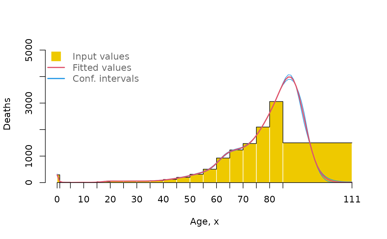

Keep that figure in mind, because the rest of the vignette is about the decisions embedded in it: the last interval’s width, the smoothing parameter, the scale of the counts, and the two kinds of interval the output carries.

What comes back

names(M1)
#> [1] "input"           "fitted"          "ci"              "goodness.of.fit"
#> [5] "smoothPar"       "bin.definition"  "deep"            "call"

element	what it holds
`input`	the arguments, as supplied. `input$x`, `input$y`, even the transformed ones.
`fitted`	the ungrouped sequence. A named vector, names are the interval labels.
`ci`	four vectors, explained under Reading the intervals.
`goodness.of.fit`	`AIC`, `BIC`, and `standard.errors` for the fitted values.
`smoothPar`	the `lambda`, `kr`, `deg` actually used.
`bin.definition`	the input and output interval boundaries, so nothing has to be rebuilt by hand.
`deep`	the internals of the fit: `C`, `B`, `dev`, `trace`, `H0`. For diagnosis.
`call`	the matched call.

summary() reports the headline numbers:

summary(M1)
#> 
#> Penalized Composite Link Model (PCLM)
#> 
#> Call:
#> pclm(x = x, y = y, nlast = nlast)
#> 
#> PCLM Type                    : Univariate
#> Number of input groups       : 19
#> Number of fitted values      : 111
#> Length of estimate bins      : 1
#> Smoothing parameter lambda   : 0.1
#> B-splines intervals/knot (kr): 2
#> B-splines degree (deg)       : 3
#> AIC                          : 39.97
#> BIC                          : 59.81

and fitted(), residuals() and plot() are the generics you would expect. residuals() returns the difference between the observed coarse count and the estimate re-aggregated to the coarse grid, so it lives on the input scale:

head(residuals(M1), 5)
#>      [0,1)      [1,5)     [5,10)    [10,15)    [15,20) 
#>  1.7450551 -2.3533494  0.9786581 -0.6128607  0.3888687
max(abs(residuals(M1)))
#> [1] 2.353349

A maximum absolute residual of about 2.4 deaths on a bin of 294 is a good sign, and it is the honest reading of what the penalty does: the fit smooths through the observation rather than interpolating it. Note that residuals are available for counts only. With an offset the fit is on the rate scale and residuals() refuses rather than returning something that looks meaningful and is not.

The width of the last interval

nlast is the one input the data cannot supply. Get it wrong and the tail is wrong, so it is worth stating plainly what the argument means.

For the Swedish male deaths used throughout, the last observed interval starts at 85. If that interval is really 85+ with everyone dying by 111, then nlast = 26. If the table was compiled with an upper bound of 95, nlast = 10. The package cannot tell, and will happily produce a smooth curve under either assumption.

omega exists to say the same thing from the other end, which is often the natural way to state it: not “the last interval is 26 years wide” but “the distribution closes at age 111”.

M_omega <- pclm(x = x, y = y, omega = 111, control = list(lambda = 100))
M_nlast <- pclm(x = x, y = y, nlast = 26,  control = list(lambda = 100))
all.equal(unname(fitted(M_omega)), unname(fitted(M_nlast)))
#> [1] TRUE

The two calls agree exactly. They are alternatives, and the package refuses both and neither:

pclm(x = x, y = y, nlast = 26, omega = 111)  # both given
#> Error:
#> ! supply 'nlast' or 'omega', not both
pclm(x = x, y = y)                           # neither given
#> Error:
#> ! supply either 'nlast' or 'omega'
pclm(x = x, y = y, omega = 85)               # not past max(x)
#> Error:
#> ! 'omega' must be greater than max(x)

A wide-open final interval is where the model has the least to work with, and the estimated tail is the most fragile part of any result. If the raw data are available at a finer resolution for the last interval, use them.

Choosing the resolution of the output

out.step sets the width of the output intervals, anywhere from 0.1 to 1. The default is 1, one-year intervals for age data.

M2 <- pclm(x = x, y = y, nlast = nlast, out.step = 0.5)
length(fitted(M2))
#> [1] 222
head(names(fitted(M2)), 4)
#> [1] "[0,0.5)" "[0.5,1)" "[1,1.5)" "[1.5,2)"

Twice as many values, half as wide, and the same total mass:

c(same_mass = all.equal(sum(fitted(M2)), sum(y)))
#> same_mass 
#>      TRUE

out.step changes the resolution of the reporting grid, not the amount of information. Asking for 0.5 does not recover the within-year structure that one-year bins never recorded; it interpolates the fitted curve at a finer spacing. Use it to line the output up with another data source, not in the hope that a smaller number makes the estimate sharper.

If the requested step does not divide the total span evenly, the last interval is widened by a hair and you are told, together with the nearby values that would have divided cleanly:

M2b <- pclm(x = x, y = y, nlast = nlast, out.step = 0.32,
            control = list(lambda = 100))
#> Warning: 'nlast' has been adjusted in order to obtain 347 bins of equal length
#> as specified in 'out.step = 0.32'. Now 'nlast = 26.04'. The impact in results
#> should be insignificant. However, if the adjustment is not acceptable try out
#> one of the following 'out.step' values: 0.1, 0.2, 0.25, 0.37, 0.5, 0.6, 0.74,
#> 0.75, 1.

suggest.valid.out.step(max(x) + nlast - min(x))
#> [1] 0.10 0.20 0.25 0.37 0.50 0.60 0.74 0.75 1.00

What a penalty buys

The single most useful sanity check is to compare the PCLM fit against the uniform spread, which is what you get with no model at all. We can build the ground truth here because the bundled data set holds deaths by single year of age, so we can aggregate to coarse bins, ungroup with each method, and see which one gets back to the truth.

# Average years lived, from a vector of deaths by single year of age.
e0 <- function(dx) {
  n <- length(dx)
  l <- rev(cumsum(rev(dx)))
  l <- l / l[1]
  L <- c((l[-1] + l[-n]) / 2, l[n])
  sum(L) / l[1]
}

# Aggregate single-age deaths into the same coarse bins used above.
grp <- rep(x, c(diff(x), nlast))
bin_deaths <- function(j) {
  as.numeric(tapply(as.numeric(ungroup.data$Dx[, j]), grp, sum))
}

For one year, 1980:

truth <- as.numeric(ungroup.data$Dx[, 1])
coarse <- bin_deaths(1)
widths <- c(diff(x), nlast)

uniform <- rep(coarse / widths, times = widths)
fit1980 <- pclm(x, coarse, nlast, control = list(lambda = 100))

round(c(truth     = e0(truth),
        uniform   = e0(uniform),
        pclm      = e0(unname(fitted(fit1980)))), 3)
#>   truth uniform    pclm 
#>  73.493  75.164  73.518

The uniform spread overstates life expectancy by more than one and a half years. PCLM lands within about two hundredths. Across all 35 years in the data set the difference is systematic rather than lucky:

errors <- t(vapply(1:35, function(j) {
  truth  <- as.numeric(ungroup.data$Dx[, j])
  coarse <- bin_deaths(j)
  uniform <- rep(coarse / widths, times = widths)
  fit <- pclm(x, coarse, nlast, control = list(lambda = 100))
  c(uniform = e0(uniform) - e0(truth),
    pclm    = e0(unname(fitted(fit))) - e0(truth))
}, numeric(2)))

round(apply(abs(errors), 2, function(z) c(mean = mean(z), max = max(z))), 3)
#>      uniform  pclm
#> mean   2.493 0.045
#> max    3.099 0.177

plot(1980:2014, errors[, "uniform"], type = "b", pch = 19, col = "grey60",
     ylim = range(errors) * 1.1,
     xlab = "Year", ylab = "Error in e0, years")
lines(1980:2014, errors[, "pclm"], type = "b", pch = 19, col = 2)
abline(h = 0, lty = 3)
legend("topleft", legend = c("uniform spread", "pclm"),
       col = c("grey60", 2), lty = 1, pch = 19, bty = "n")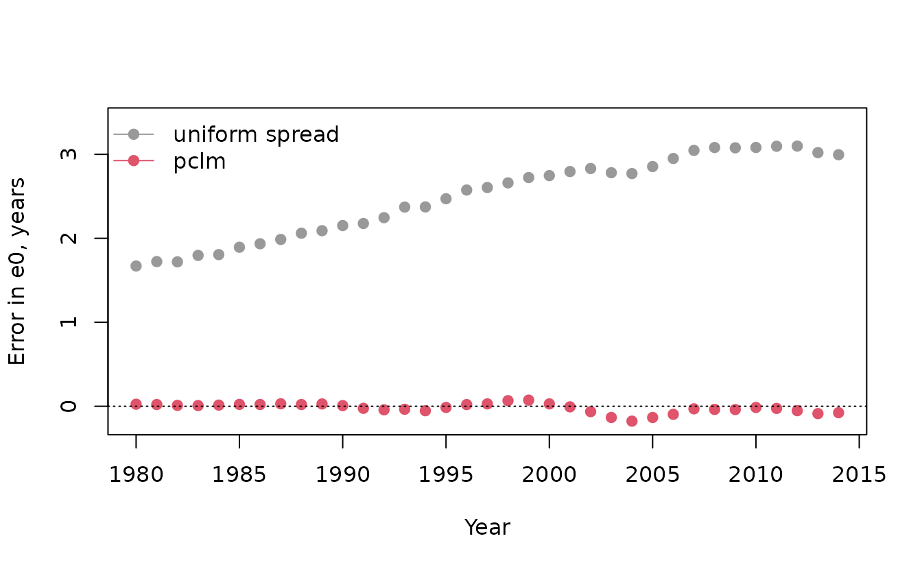

The uniform spread is biased upward by 2.5 years on average and by more than three in the worst year, always in the same direction: flat bins put too much mass at the young end of every interval, including the open one. The PCLM error averages under a tenth of a year.

The smoothing parameter

lambda is the knob that decides how much structure the estimate is allowed to have. Too small and the fit chases noise and the artificial wiggles introduced by the bin edges; too large and real features flatten out. Here is the Old Faithful geyser, 272 eruptions binned into four one-minute intervals (Azzalini and Bowman 1990). The data have nothing to do with mortality, which is the point: nothing in the model is demographic.

faithful_counts <- hist(datasets::faithful$eruptions,
                        breaks = seq(1.5, 5.5, by = 1),
                        plot   = FALSE)$counts
faithful_counts
#> [1]  92  14 109  57

Mf <- pclm(x = 1.5:4.5, y = faithful_counts, nlast = 1,
           out.step = 0.1)
Mf$smoothPar[1]
#>   lambda 
#> 65.22826

plot(Mf, xlab = "Eruption length, minutes", ylab = "Eruptions")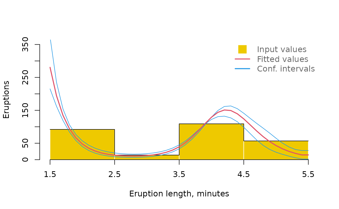

Two modes, and they are real: geologists classify Old Faithful eruptions as short or long. The dip between them is the feature to watch, since it is what a penalty that is too heavy will erase first.

valley <- function(L) {
  fv <- as.numeric(fitted(pclm(1.5:4.5, faithful_counts, 1, out.step = 0.1,
                               control = list(lambda = L))))
  round(c(valley = min(fv[11:20]), peak = max(fv)), 2)
}
rbind(lambda_1   = valley(1),
      lambda_auto = valley(Mf$smoothPar[1]),
      lambda_1e6  = valley(1e6))
#>             valley  peak
#> lambda_1      0.98 29.25
#> lambda_auto   1.10 28.05
#> lambda_1e6    5.21 10.76

At lambda = 1e6 the valley is nearly gone, its minimum lifted from about 1 to 5 eruptions per 0.1-minute cell. The automatic choice sits between the two extremes, and the ordering of BIC agrees that it is the better compromise:

sapply(c(1, Mf$smoothPar[1], 1e6), function(L) {
  M <- pclm(1.5:4.5, faithful_counts, 1, out.step = 0.1,
            control = list(lambda = L))
  round(c(BIC = BIC(M), AIC = AIC(M)), 2)
})
#>          lambda      
#> BIC 7.94   7.65 70.33
#> AIC 9.87   9.45 71.51

Two cautions about letting the package choose. First, the search interval is finite, int.lambda defaults to c(0.1, 1e5), and the optimum does sometimes land on the boundary. When it does, the answer is the boundary value rather than the true optimum:

M_auto <- pclm(x, y, nlast, control = list(lambda = NA))
M_wide <- pclm(x, y, nlast,
               control = list(lambda = NA, int.lambda = c(1e-4, 1e5)))
c(default_search = M_auto$smoothPar[1], wider_search = M_wide$smoothPar[1])
#> default_search.lambda   wider_search.lambda 
#>              0.100000              0.083597

Second, select with BIC (the default) unless you have a reason not to (Hastie and Tibshirani 1990). It penalizes complexity harder and is the safer choice for a distribution where a spurious bump in the tail is costly. AIC will occasionally prefer a visibly wiggly fit.

Both criteria, and the fitted values themselves, are returned so the choice can be checked rather than trusted:

M_bic <- pclm(x, y, nlast, control = list(lambda = NA, opt.method = "BIC"))
M_aic <- pclm(x, y, nlast, control = list(lambda = NA, opt.method = "AIC"))
c(bic_choice = M_bic$smoothPar[1],
  aic_choice = M_aic$smoothPar[1])
#> bic_choice.lambda aic_choice.lambda 
#>               0.1               0.1

Fixing lambda by hand is much faster than searching, roughly a factor of thirty on this example, so once a value is known to work it is worth passing it in. The full set of fitting controls is in ?control.pclm.

Estimating rates, not counts

Pass an offset and the model estimates a rate rather than a count. The offset is the population exposed to risk, one value per input bin, and it is ungrouped internally on the same grid so the fitted rates line up with the fitted counts.

Ex <- c(114, 440, 509, 492, 628, 618, 576, 580, 634, 657,
        631, 584, 573, 619, 530, 384, 303, 245, 249) * 1000

M3 <- pclm(x = x, y = y, nlast = nlast, offset = Ex)
fitted(M3)[1:5]
#>        [0,1)        [1,2)        [2,3)        [3,4)        [4,5) 
#> 2.478299e-03 4.098609e-04 1.051348e-04 4.515452e-05 3.275430e-05

The values are now central death rates on a log scale when plotted:

plot(M3, type = "s", xlab = "Age, x", ylab = "m(x), log scale")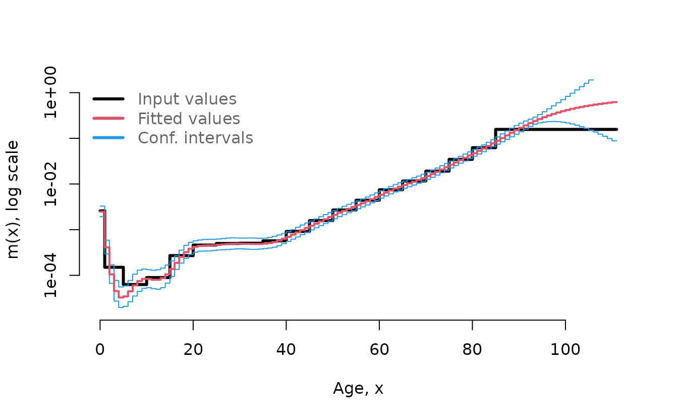

There are two accepted forms, and they give slightly different answers.

Exposures on the coarse grid, the same length as y. This is the usual case and the one to reach for. The exposures are ungrouped inside the model, on the same fine grid as the counts.
Exposures already ungrouped, the same length as the output. They are then taken as fixed, which is what you want when the exposures come from a source with a genuinely finer resolution.

Ex_fine <- fitted(pclm(x = x, y = Ex, nlast = nlast))   # 111 values

M_coarse <- pclm(x = x, y = y, nlast = nlast, offset = Ex)
M_fine   <- pclm(x = x, y = y, nlast = nlast, offset = Ex_fine)

# Same rates to within a few percent through the bulk of the distribution,
# and further apart in the extreme tail where the counts are thin.
round(range(fitted(M_fine) / fitted(M_coarse)), 3)
#> [1] 1.023 1.508

Do not mix them up: the two lengths mean different things and both are accepted, so a mistake here produces a plausible curve rather than an error.

Small counts and zeros

Poisson counts of zero are informative, and in the extreme ages they are also routine. The model handles them, but tiny counts make a large response to a small change, so the package warns and suggests a fix.

small <- c(0, 0, 1, 0, 2, 1, 0, 3, 2, 1)
M_small <- pclm(x = 0:9, y = small, nlast = 1,
                control = list(lambda = 10))
#> Input data contains zeros. Replace zero values with a very small number to avoid erroneous results. If the input data contains small values, you might also want to transform it for the purpose of ungrouping. E.g. Multiplication by 100.

Multiplying by a constant is the recommended move. It changes nothing about the relative fit, because the penalty acts on the spline coefficients and the Poisson likelihood absorbs the scale, but it keeps the internal arithmetic away from underflow in the tail:

M_scaled <- pclm(x = 0:9, y = small * 100, nlast = 1,
                 control = list(lambda = 10))
#> Input data contains zeros. Replace zero values with a very small number to avoid erroneous results. If the input data contains small values, you might also want to transform it for the purpose of ungrouping. E.g. Multiplication by 100.
c(total_in   = sum(small * 100),
  total_out  = sum(fitted(M_scaled)),
  head_fit   = round(head(fitted(M_scaled), 3), 1))
#>       total_in      total_out head_fit.[0,1) head_fit.[1,2) head_fit.[2,3) 
#>       1000.000       1000.001          4.900         16.700         44.200

Reading the intervals

The ci element holds four vectors and they are not interchangeable. Getting this wrong is the easiest way to publish a wrong statement, so it is worth being precise.

names(M1$ci)
#> [1] "upper"      "lower"      "conf_lower" "conf_upper"

lower and upper are scenarios, not bounds. They answer a specific question: what does the distribution look like if everyone’s hazard is uniformly lower (or higher)? The curves are built by scaling the whole hazard, then rescaled so that each scenario still totals sum(fitted). That mass constraint is what makes them useful as low and high inputs to a life table, and also what makes them cross the point estimate in the tail: the low scenario has the same total mass but pushes it toward older ages, so past some age it lies above the fit.

diff <- fitted(M1) - M1$ci$lower
c(totals_equal = isTRUE(all.equal(sum(M1$ci$lower), sum(y))),
  first_age_above = names(fitted(M1))[min(which(diff < 0))])
#>    totals_equal first_age_above 
#>          "TRUE"       "[81,82)"

conf_lower and conf_upper are pointwise intervals around each fitted value, at the level given by ci.level (default 95). They always bracket the estimate, and they do not total anything in particular.

i <- c(1, 30, 70, 100, 111)
data.frame(
  bin       = names(fitted(M1))[i],
  fitted    = round(fitted(M1)[i], 1),
  conf_lo   = round(M1$ci$conf_lower[i], 1),
  conf_up   = round(M1$ci$conf_upper[i], 1),
  scen_lo   = round(M1$ci$lower[i], 1),
  scen_up   = round(M1$ci$upper[i], 1)
)
#>                 bin fitted conf_lo conf_up scen_lo scen_up
#> [0,1)         [0,1)  292.3   260.7   327.6   261.2   327.6
#> [29,30)     [29,30)   58.3    51.6    65.8    51.8    65.7
#> [69,70)     [69,70) 1294.3  1260.4  1329.0  1275.7  1314.4
#> [99,100)   [99,100)  419.0   278.0   631.6   452.8   356.0
#> [110,111) [110,111)    1.8     0.3    10.7    27.9     0.0

Read the last three rows: at ages 99 and above the scenario lower curve sits above the fit, while the pointwise interval still brackets it. Two different objects, two different jobs.

lo <- M1$ci$conf_lower
up <- M1$ci$conf_upper
f  <- fitted(M1)
age <- seq(0, 110, length.out = length(f))

plot(age, f, type = "l", lwd = 2, ylim = c(0, max(up) * 1.05),
     xlab = "Age, x", ylab = "Deaths")
polygon(c(age, rev(age)), c(lo, rev(up)),
        col = adjustcolor("steelblue", 0.25), border = NA)
lines(age, f, lwd = 2)
lines(age, M1$ci$lower, lwd = 2, lty = 2, col = 2)
lines(age, M1$ci$upper, lwd = 2, lty = 2, col = 2)
legend("topright", bty = "n", lty = c(1, 1, 2), lwd = 2,
       col = c(1, "steelblue", 2),
       legend = c("fitted", "pointwise 95%", "mass-preserving scenarios"))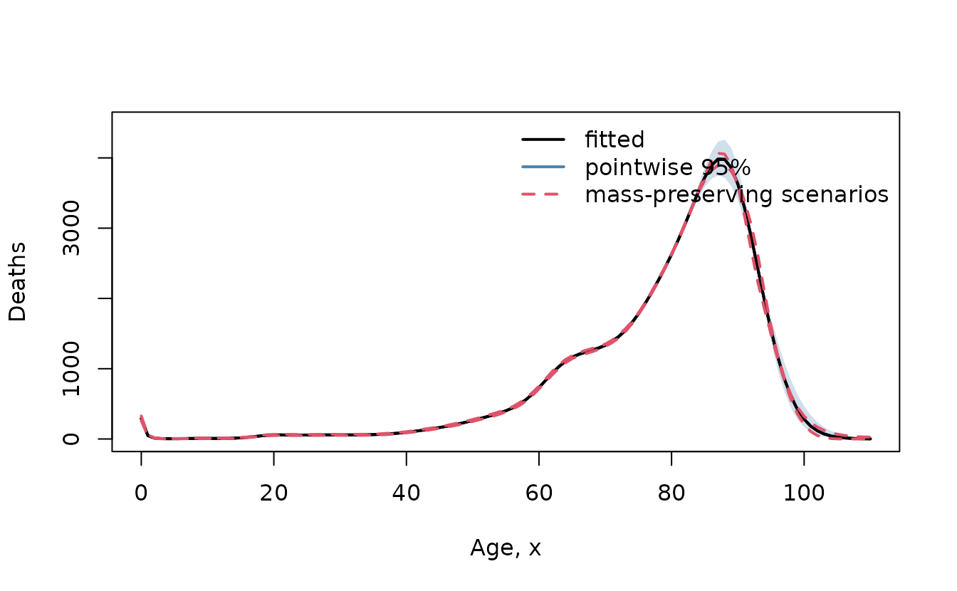

Neither interval covers the region where nothing was observed in the sense of a sampling guarantee; see the next section. Both are computed from the sandwich estimator of the spline coefficients and inherit its assumptions, one of which is that the model is correctly specified.

Missing data and an open interval that moves

Two problems in published data led to the na.action argument, and both are common enough to deserve a worked example.

The first is an open age group that changes over time. A country may close its tables at 65+ for a few years, then at 80+, then at 85+. For a two-dimensional fit the surface has to be rectangular, so the cells above the early ceiling are simply unobserved.

grp2 <- rep(x, c(diff(x), nlast))
years <- 1:12
y2d <- aggregate(ungroup.data$Dx[, years], by = list(grp2), FUN = "sum")[, -1]

# The top of the surface is unobserved in the early years: the oldest ages
# were folded into the open interval at a lower ceiling then.
y_ragged <- y2d
y_ragged[17:19, 1:4] <- NA
y_ragged[c(1:3, 16:19), 1:5]
#>     1980  1981  1982  1983  1984
#> 1    671   653   635   646   601
#> 2    141   101   126   101    87
#> 3    116   102    91    93    78
#> 16 13168 13352 12948 12713 12399
#> 17    NA    NA    NA    NA 16267
#> 18    NA    NA    NA    NA 16426
#> 19    NA    NA    NA    NA 20271

The default na.action = "fail" rejects it, exactly as the package always did:

pclm2D(x = x, y = y_ragged, nlast = nlast, verbose = FALSE)
#> Error:
#> ! 'y' contains NA values. Use na.action = "omit" to smooth over them.

na.action = "omit" drops those cells from the likelihood and lets the penalty bridge the gap. The output grid is untouched, so the surface comes back whole.

P_ragged <- pclm2D(x = x, y = y_ragged, nlast = nlast,
                   na.action = "omit", verbose = FALSE,
                   control = list(lambda = c(1, 1), kr = 5))
dim(fitted(P_ragged))
#> [1] 111  12
all(is.finite(fitted(P_ragged)))
#> [1] TRUE

The second problem is a year with no exposure. Deaths recorded annually, population only every third year, which is the case that prompted issue #6.

Ex2d <- aggregate(ungroup.data$Ex[, years], by = list(grp2), FUN = "sum")[, -1]
Ex2d[, c(2, 3, 5, 6, 8, 9, 11, 12)] <- NA

Omission applies to the offset too, so the same call recovers a rate in every year:

P_missing <- pclm2D(x = x, y = y2d, nlast = nlast, offset = Ex2d,
                    na.action = "omit", verbose = FALSE,
                    control = list(lambda = c(1, 1), kr = 5))
dim(fitted(P_missing))
#> [1] 111  12
all(is.finite(fitted(P_missing)))
#> [1] TRUE

Two things to be honest about. Only NA counts as unobserved; Inf remains an error under "omit", so “missing” and “invalid” stay distinguishable. And an interpolated year is an estimate from its neighbours, borrowing strength from both axes. It is not a recovered measurement, and the confidence intervals around it are as wide as the penalty allows and no wider.

The totals make the same point. With every cell observed the fit conserves mass exactly, but under omission the gaps are filled in by the penalty and the fitted total exceeds the observed one:

c(
  observed_cells   = sum(y_ragged, na.rm = TRUE),
  fitted_all_cells = sum(fitted(P_ragged))
)
#>   observed_cells fitted_all_cells 
#>           910351          1096740

Two dimensions

The model extends to a surface. pclm2D ungroups coarse age distributions for several adjacent years at once and smooths across them, so the age profile borrows strength from neighbouring years and the time trend borrows strength from neighbouring ages. This is the setting of Rizzi et al. (2019) and, as the previous section showed, the setting where data are most often ragged.

The input response is a matrix or data frame: rows are age intervals, columns are years, with the same x and nlast as before.

years10 <- 1:10
y10  <- aggregate(ungroup.data$Dx[, years10], by = list(grp2), FUN = "sum")[, -1]
Ex10 <- aggregate(ungroup.data$Ex[, years10], by = list(grp2), FUN = "sum")[, -1]
dim(y10)
#> [1] 19 10

P_counts <- pclm2D(x = x, y = y10, nlast = nlast, verbose = FALSE,
                   control = list(lambda = c(1, 1), kr = 5))
dim(fitted(P_counts))
#> [1] 111  10

P_rates <- pclm2D(x = x, y = y10, nlast = nlast, offset = Ex10,
                  verbose = FALSE, control = list(lambda = c(1, 1), kr = 5))
summary(P_rates)
#> 
#> Penalized Composite Link Model (PCLM)
#> 
#> Call:
#> pclm2D(x = x, y = y10, nlast = nlast, offset = Ex10, verbose = FALSE, 
#>     control = list(lambda = c(1, 1), kr = 5))
#> 
#> PCLM Type                    : Two-Dimensional
#> Number of input groups       : 19 x 10
#> Number of fitted values      : 111 x 10
#> Dimension of estimate bins   : 1 x 1
#> Smoothing parameter lambda   : 1 x 1
#> B-splines intervals/knot (kr): 5
#> B-splines degree (deg)       : 3
#> AIC                          : 1060.05
#> BIC                          : 1267.3

Note kr = 5 in both calls. This matters. The default for pclm2D is kr = 7, and kr sets how many values along an axis share one spline interval, so a panel with fewer than seven years leaves the year axis with no internal knot at all. The package now says so instead of failing deep in the basis construction:

pclm2D(x = x, y = y10[, 1:5], nlast = nlast, verbose = FALSE,
       control = list(lambda = c(1, 1)))
#> Error:
#> ! 'kr' = 7 is too large for the year axis of length 5. At least one internal knot is required, so use kr <= 5.

kr is the main cost knob for the two-dimensional fit, since it fixes the number of spline coefficients in each direction. A smaller kr means more coefficients, a more flexible fit, and a slower one:

basis_size <- vapply(c(2, 3, 5, 7), function(k) {
  P <- pclm2D(x = x, y = y10, nlast = nlast, verbose = FALSE,
              control = list(lambda = c(1, 1), kr = k))
  ncol(P$deep$B)
}, numeric(1))
setNames(basis_size, paste0("kr=", c(2, 3, 5, 7)))
#> kr=2 kr=3 kr=5 kr=7 
#>  472  240  125   76

That is the number of coefficients the penalty is applied to, and it drives both the flexibility and the runtime.

plot(P_counts, xlab = "Age", ylab = "Year", zlab = "Deaths")

plot(P_rates, xlab = "Age", ylab = "Year", zlab = "log m(x)")

The observed input can be plotted on the same axes, which is the honest comparison, because it shows how much of the picture is the data and how much is the smoother:

plot(P_counts, type = "observed", xlab = "Age", ylab = "Year",
     zlab = "Deaths per year of age")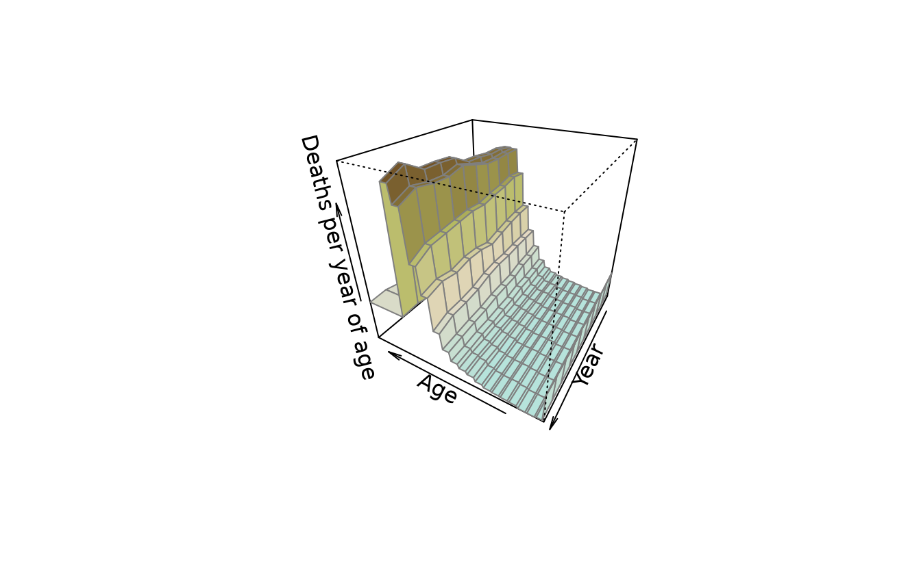

The plot method takes phi and theta for the viewing angle, nbcol and colors for the palette, and passes anything else to persp(). If the rotated view is awkward in a static document, extract the matrix and plot it flat:

Z <- fitted(P_rates)
image(x = as.numeric(sub("^\\[([0-9.]+),.*$", "\\1", rownames(Z))),
      y = years10, z = log(Z), col = hcl.colors(64, "YlOrBr", rev = TRUE),
      xlab = "Age, x", ylab = "Year")
contour(x = as.numeric(sub("^\\[([0-9.]+),.*$", "\\1", rownames(Z))),
        y = years10, z = log(Z), add = TRUE, col = "grey30", labcex = 0.7)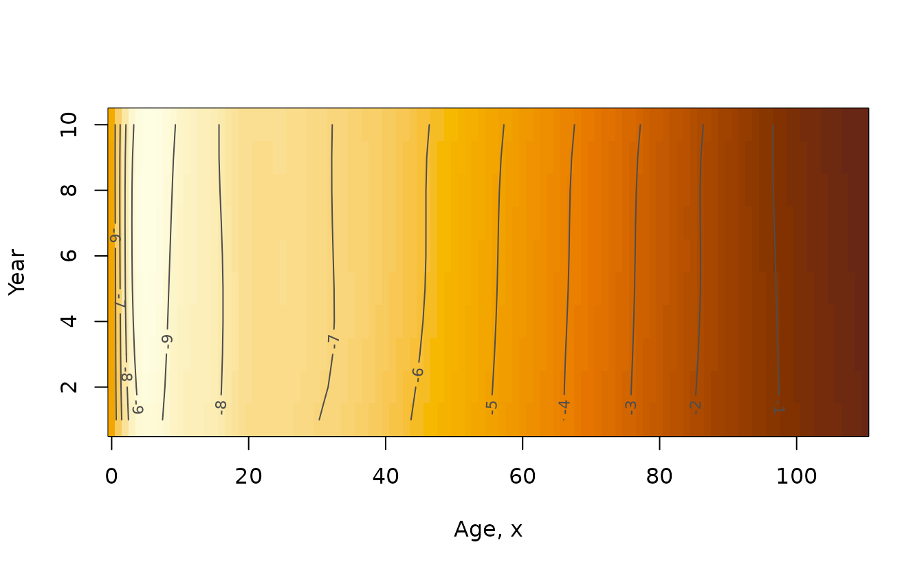

Cost

The two-dimensional fit is meaningfully slower than the one-dimensional one, and it is worth knowing the shape of the cost before pointing it at a large panel. Roughly:

the fit is iterative per column of the surface, so cost grows close to linearly in the number of years;
a smaller kr multiplies that by enlarging the basis;
fitting rates costs several times what fitting counts does, because the offset is itself ungrouped with a full one-dimensional fit on each column;
asking for lambda = c(NA, NA) starts a search over two parameters and can take minutes on a wide surface.

For interactive work, fix lambda, and choose kr from the panel size. The default kr = 7 is a reasonable compromise for a surface spanning decades; shorten it for a handful of years.

How to get it wrong

Three traps, all of which produce output that looks fine.

Passing the wrong nlast. Nothing detects it, and the whole tail is wrong. If the estimate at the oldest ages looks implausible, this is the first thing to check.

Treating ci$lower and ci$upper as a confidence band. They are mass-preserving scenarios and they cross the fit. Use conf_lower and conf_upper for an error bar, lower and upper as life table inputs.

Reading a fine out.step as extra information. It is interpolation of the fitted curve. The information content is set by the input bins.

To these we can add the statistical caveats that come with any penalized likelihood: the intervals rely on the model being right, the choice of lambda is data-driven and so the coverage is approximate, and the estimate in a region that was never observed is extrapolation from the penalty alone.

Where to go next

?pclm and ?pclm2D document every argument and the full return value.
?control.pclm and ?control.pclm2D list the fitting controls and their defaults.
Rizzi et al. (2015) is the reference for the one-dimensional method, Rizzi et al. (2019) for the two-dimensional extension with time, and Eilers (2007) for the penalized-likelihood machinery. Rizzi et al. (2016) compares ungrouping methods against one another.
The MortalityLaws package downloads mortality data from the Human Mortality Database in a form that can be fed straight into pclm.

sessionInfo()
#> R version 4.6.1 (2026-06-24)
#> Platform: x86_64-pc-linux-gnu
#> Running under: Ubuntu 24.04.5 LTS
#> 
#> Matrix products: default
#> BLAS:   /usr/lib/x86_64-linux-gnu/openblas-pthread/libblas.so.3 
#> LAPACK: /usr/lib/x86_64-linux-gnu/openblas-pthread/libopenblasp-r0.3.26.so;  LAPACK version 3.12.0
#> 
#> locale:
#>  [1] LC_CTYPE=C.UTF-8       LC_NUMERIC=C           LC_TIME=C.UTF-8       
#>  [4] LC_COLLATE=C.UTF-8     LC_MONETARY=C.UTF-8    LC_MESSAGES=C.UTF-8   
#>  [7] LC_PAPER=C.UTF-8       LC_NAME=C              LC_ADDRESS=C          
#> [10] LC_TELEPHONE=C         LC_MEASUREMENT=C.UTF-8 LC_IDENTIFICATION=C   
#> 
#> time zone: UTC
#> tzcode source: system (glibc)
#> 
#> attached base packages:
#> [1] stats     graphics  grDevices utils     datasets  methods   base     
#> 
#> other attached packages:
#> [1] ungroup_1.6.3
#> 
#> loaded via a namespace (and not attached):
#>  [1] vctrs_0.7.3       cli_3.6.6         knitr_1.52        rlang_1.3.0      
#>  [5] xfun_0.61         otel_0.2.0        textshaping_1.0.5 jsonlite_2.0.0   
#>  [9] glue_1.8.1        htmltools_0.5.9   ragg_1.5.2        sass_0.4.10      
#> [13] rmarkdown_2.32    grid_4.6.1        evaluate_1.0.5    jquerylib_0.1.4  
#> [17] fastmap_1.2.0     yaml_2.3.12       lifecycle_1.0.5   compiler_4.6.1   
#> [21] fs_2.1.0          Rcpp_1.1.2        pbapply_1.7-5     lattice_0.22-9   
#> [25] systemfonts_1.3.2 digest_0.6.39     R6_2.6.1          pillar_1.11.1    
#> [29] parallel_4.6.1    Rdpack_2.6.6      rbibutils_2.4.1   Matrix_1.7-5     
#> [33] bslib_0.12.0      tools_4.6.1       pkgdown_2.2.1     cachem_1.1.0     
#> [37] desc_1.4.3

References

Azzalini, Adelchi, and Adrian W Bowman. 1990. “A Look at Some Data on the Old Faithful Geyser.” Applied Statistics 39 (3): 357–65. https://doi.org/10.2307/2347385.

Eilers, Paul HC. 2007. “Ill-Posed Problems with Counts, the Composite Link Model and Penalized Likelihood.” Statistical Modelling 7 (3): 239–54. https://doi.org/10.1177/1471082X0700700302.

Hastie, Trevor J, and Robert J Tibshirani. 1990. “Generalized Additive Models.” Monographs on Statistics and Applied Probability 43.

Rizzi, Silvia, Jutta Gampe, and Paul H. C. Eilers. 2015. “Efficient Estimation of Smooth Distributions from Coarsely Grouped Data.” American Journal of Epidemiology 182 (2): 138–47. https://doi.org/10.1093/aje/kwv020.

Rizzi, Silvia, Ulrich Halekoh, Mikael Thinggaard, et al. 2019. “How to Estimate Mortality Trends from Grouped Vital Statistics.” International Journal of Epidemiology 48 (2): 571–82. https://doi.org/10.1093/ije/dyy183.

Rizzi, Silvia, Mikael Thinggaard, Gerda Engholm, et al. 2016. “Comparison of Non-Parametric Methods for Ungrouping Coarsely Aggregated Data.” BMC Medical Research Methodology 16 (1): 59. https://doi.org/10.1186/s12874-016-0157-8.

Thompson, R, and RJ Baker. 1981. “Composite Link Functions in Generalized Linear Models.” Applied Statistics, 125–31.

Ungrouping binned count data with the penalized composite link model

Marius D. Pascariu, Maciej J. Dańko, Jonas Schöley and Silvia Rizzi

2026-10-02