Two-Dimensional Penalized Composite Link Model (PCLM-2D)

Fit two-dimensional penalized composite link model (PCLM-2D), e.g. simultaneous ungrouping of age-at-death distributions grouped in age classes for adjacent years. The PCLM can be extended to a two-dimensional regression problem. This is particularly suitable for mortality analysis when mortality surfaces are to be estimated to capture both age-specific trajectories of coarsely grouped distributions and time trends (Rizzi et al. 2019) .

Usage

pclm2D(
  x,
  y,
  nlast = NULL,
  offset = NULL,
  out.step = 1,
  ci.level = 95,
  verbose = TRUE,
  control = list(),
  omega = NULL,
  na.action = c("fail", "omit")
)

Arguments

x: Vector containing the starting values of the input intervals/bins. For example: if we have 3 bins [0,5), [5,10) and [10, 15), x will be defined by the vector: c(0, 5, 10).
y: data.frame with counts to be ungrouped. The number of rows should be equal with the length of x.
nlast: Length of the last interval. In the example above nlast would be 5.
offset: Optional offset term to calculate smooth mortality rates. A vector of the same length as x and y, or one of the same length as the ungrouped output. See Rizzi et al. (2015) for further details.
out.step: Length of estimated intervals in output. Values between 0.1 and 1 are accepted. Default: 1.
ci.level: Confidence level, as a percentage rather than a proportion, so 95 and not 0.95. Values in [50.1, 99.9] are accepted. It sets the width of both interval pairs in ci: the pointwise conf_lower and conf_upper, and the mass-preserving lower and upper scenarios. Default: 95.
verbose: Logical value. Indicates whether a progress bar should be shown or not. Default: TRUE.
control: List of fitting controls, given by name. A misspelled entry is an error rather than being silently ignored. An unnamed entry is matched positionally, so list(100) sets lambda and nothing else; naming every entry is strongly preferred. Any setting not supplied takes its default from control.pclm for this function, or control.pclm2D for pclm2D. See those pages for the meaning and default of each of lambda, kr, deg, int.lambda, diff, opt.method, max.iter and tol.
omega: Closing age of the distribution. An alternative to nlast: when it is given, the width of the last interval is taken as omega - max(x). Give one of the two, not both.
na.action: What to do with unobserved cells in y. "fail", the default, rejects them. "omit" drops the matching rows and lets the smoothing penalty bridge the gap, which is how a surface with interior gaps or a missing year is handled. Only NA counts as unobserved; infinite values are always an error.

Value

The output is a list with the following components:

input: A list with arguments provided in input. Saved for convenience.
fitted: The fitted values of the PCLM model.
ci: A list with two kinds of interval and they are not interchangeable. lower and upper are the two mass-conserving scenarios: the distribution implied by a uniformly lower and a uniformly higher hazard, each rescaled so that it totals sum(fitted). Because the total is held fixed, the low scenario moves deaths towards older ages and the two curves cross fitted in the tail. They are therefore scenarios, not pointwise bounds, and they carry no coverage level. conf_lower and conf_upper are the pointwise marginal ci.level interval for the fitted values, computed as fitted * exp(-/+ qnorm * SE). These do satisfy conf_lower <= fitted <= conf_upper and they do not total sum(fitted). Use the first pair as low and high inputs to a life table, the second as a pointwise error bar on the estimate.
goodness.of.fit: A list containing goodness of fit measures: standard errors, AIC and BIC.
smoothPar: Estimated smoothing parameters. In the univariate model a named vector of lambda, kr and deg. In the two-dimensional model lambda splits into lambda.x for the age axis and lambda.y for the year axis, so the vector is lambda.x, lambda.y, kr, deg.
bin.definition: Additional values to identify the bins limits and location in input and output objects.
deep: A list of objects created in the fitting process. Useful in diagnosis of possible issues.
call: An unevaluated function call, that is, an unevaluated expression which consists of the named function applied to the given arguments.

References

Rizzi S, Gampe J, Eilers PHC (2015). “Efficient Estimation of Smooth Distributions From Coarsely Grouped Data.” American Journal of Epidemiology, 182(2), 138-147. doi:10.1093/aje/kwv020 .

Rizzi S, Halekoh U, Thinggaard M, Engholm G, Christensen N, Johannesen TB, Lindahl-Jacobsen R (2019). “How to estimate mortality trends from grouped vital statistics.” International Journal of Epidemiology, 48(2), 571–582. doi:10.1093/ije/dyy183 .

Examples

# Input data
Dx <- ungroup.data$Dx
Ex <- ungroup.data$Ex

# Aggregate data to be ungrouped in the examples below
# Select a 10y data frame
x      <- c(0, 1, seq(5, 85, by = 5))
nlast  <- 26
n      <- c(diff(x), nlast)
group  <- rep(x, n)
y      <- aggregate(Dx, by = list(group), FUN = "sum")[, 2:10]
offset <- aggregate(Ex, by = list(group), FUN = "sum")[, 2:10]

# Example 1 ---------------------- 
# Fit model and ungroup data using PCLM-2D
P1 <- pclm2D(x, y, nlast)
#>    Ungrouping data      
summary(P1)
#> 
#> Penalized Composite Link Model (PCLM)
#> 
#> Call:
#> pclm2D(x = x, y = y, nlast = nlast)
#> 
#> PCLM Type                    : Two-Dimensional
#> Number of input groups       : 19 x 9
#> Number of fitted values      : 111 x 9
#> Dimension of estimate bins   : 1 x 1
#> Smoothing parameter lambda   : 1 x 1
#> B-splines intervals/knot (kr): 7
#> B-splines degree (deg)       : 3
#> AIC                          : 1858.11
#> BIC                          : 1982

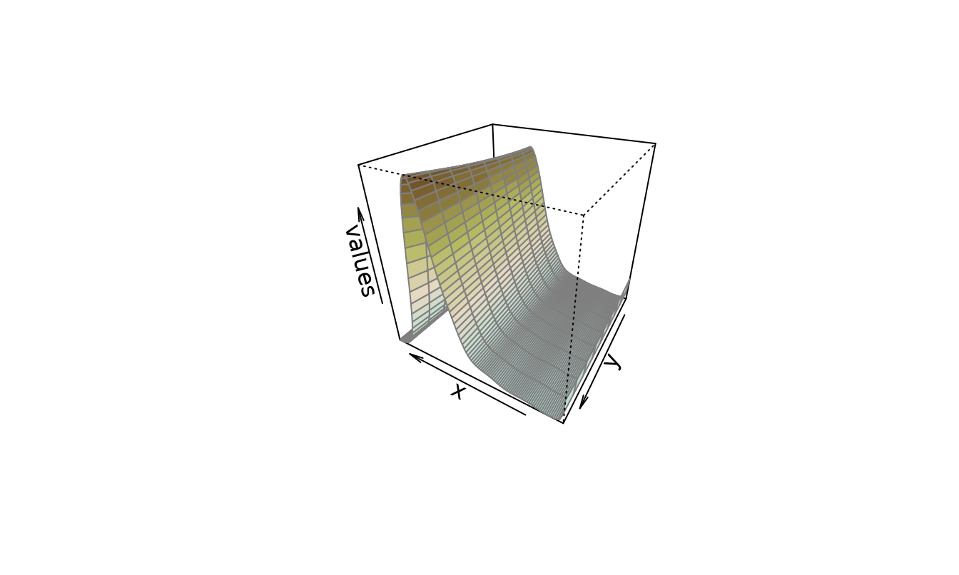
# Plot fitted values
plot(P1)


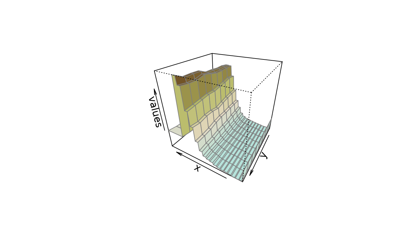
# Plot input data
plot(P1, "observed")


# NOTE: pclm2D does not search for optimal smoothing parameters by default
# (like pclm does) because it is more time consuming. If optimization is 
# required set lambda = c(NA, NA):

P1 <- pclm2D(x, y, nlast, control = list(lambda = c(NA, NA)))
#>    Optimizing lambda     Ungrouping data      

# Example 2 ---------------------- 
# Ungroup and build a mortality surface
P2 <- pclm2D(x, y, nlast, offset)
#>    Ungrouping offset   Ungrouping data      
summary(P2)
#> 
#> Penalized Composite Link Model (PCLM)
#> 
#> Call:
#> pclm2D(x = x, y = y, nlast = nlast, offset = offset)
#> 
#> PCLM Type                    : Two-Dimensional
#> Number of input groups       : 19 x 9
#> Number of fitted values      : 111 x 9
#> Dimension of estimate bins   : 1 x 1
#> Smoothing parameter lambda   : 1 x 1
#> B-splines intervals/knot (kr): 7
#> B-splines degree (deg)       : 3
#> AIC                          : 1829.16
#> BIC                          : 1952.89

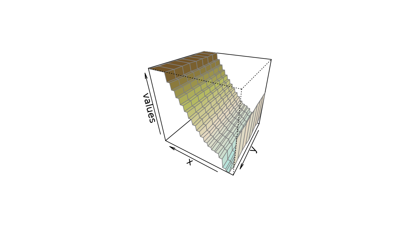
plot(P2, type = "observed")

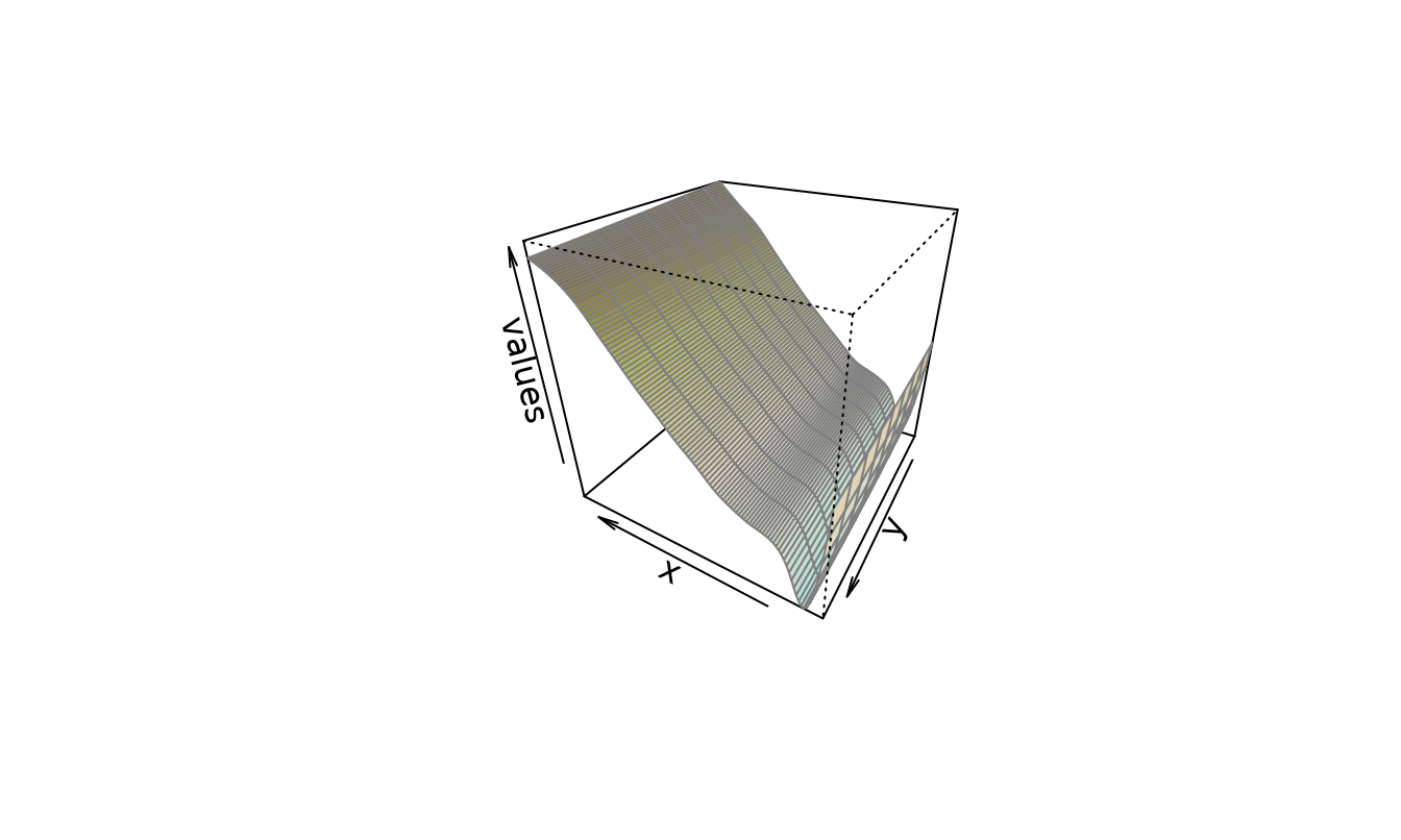
plot(P2, type = "fitted")

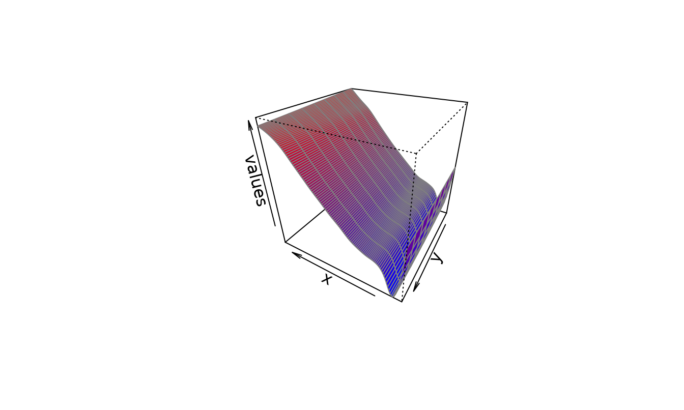
plot(P2, type = "fitted", colors = c("blue", "red"))